2020-02-27 12:28:14
Preliminaries
Announcements
- Friday February 7, 2020 - “Best Practices of Maintaining a Lab Notebook to improve Accountability”, Melissa Ishler, Ph.D. Department of Entomology, The Pennsylvania State University, 11:15 am to 12:05 pm. 127 Noll Laboratory, Host: Department of Kinesiology
- Institute for Computational and Data Science (ICDS) events
- “The Data Deluge”, ICDS Symposium, March 16-17, 2020, NLI.
Today’s agenda
- Registration
- What, why, who, how?
- Tools for reproducible workflows
- Introduction to RStudio
- Introduction to R Markdown
- Doing real work with R Markdown
Registration
Registered reports
- What are they?
- Why are they a thing?
- Who’s doing them?
- How they work and how to get involved
What are they?
- Peer review and provisional acceptance of methodologically sound study proposals
Why registered reports?
- Results (positive or null) don’t determine publication (prevent publication bias)
- Reduce questionable practices
- p-hacking
- HARKing
Why not registered reports
- Restrict creativity in reporting “un-registered”/exploratory analyses?
- Clearer communication about confirmatory vs. exploratory
- Mandatory vs. optional
- Clinical trials vs. fundamental research
- Exploration is not a dirty word
Who’s doing them?
- Journals with Registered Reports from COS
- How do they work?
- Google sheet comparing features https://docs.google.com/spreadsheets/d/1D4_k-8C_UENTRtbPzXfhjEyu3BfLxdOsn9j-otrO870/edit#gid=0

Preregistration separate from publication
AsPredicted.org
- Standardized preregistration tool
- Separate confirmatory from exploratory analyses
- One author completes checklist, others receive email to approve
- Unique (private) URL to pdf
- Share when you like or never
Your thoughts on registered reports, pregistration?
Tools for reproducible workflows
RStudio
- An integrated development environment (IDE) for R
Components of RStudio
- Code editor
- R console
- Integrated help
- Image viewer
- Integration with git and other version-control packages
- Project management
R Markdown
- Markdown
- Mark-up language to make it easy to write HTML
- R Markdown a special type of Markdown
- Allows for “literate” programming, mixing text, analysis, figures
- Adds to Markdown syntax
Let’s do this…
- Open up RStudio
- Create a new R Markdown document
File/New File/R Markdown...
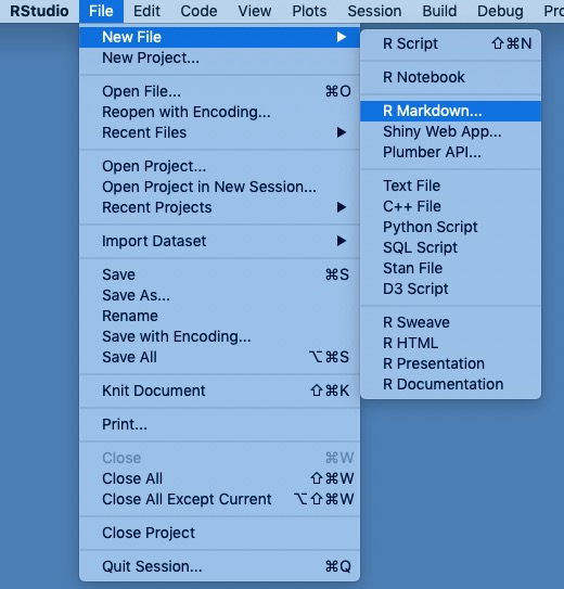
- Select
Document, call it something sensible likepsy-525-rmarkdown-testbed- NB: This is the document’s title not the name of the file.
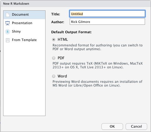
- Save the file as
testbed.Rmd
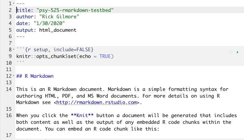
Anatomy of an R Markdown file
- Header
- Chunks
- Text, etc.
Markdown syntax
- Text formatting
- italics by surrounding text with single asterisks or underscores:
*italics*or_italics_ - boldface by surrounding text with double asterisks or underscores:
**boldface**or__boldface__
- italics by surrounding text with single asterisks or underscores:
- Text formatting
strikethroughby surrounding text with double tildes:~~strikethrough~~- Clickable URLs by surrounding link text with square brackets and URL with parentheses:
[Clickable URLs](http://www.psu.edu)
Markdown syntax
- Paragraph formatting
- Headings with level specified by the number of hash (#) marks
- Lists (bullet and enumerated)
- Block quotes
- Code blocks
# This is a Heading 1
## This is a Heading 2
### This is a Heading 3
Code:
- An item
    - A nested item
        - A doubly-nested item
- Another item
- An item
- A nested item
- A doubly-nested item
- A nested item
- Another item
Code:
1. An enumerated item
    - A nested item
1. A second enumerated item
- An enumerated item
- A nested item
- A second enumerated item
Notice how the numbers are incremented automatically!
Learn from my mistakes…
<CTRL>+2goes to console<CTRL>+1goes to source<UP-ARROW><RETURN><COMMAND><ALT>+I(Mac OS);<CTRL><ALT>+I(Windows) inserts a chunk- Train your fingers now!
Code:
> Four score and seven years ago, some famous President
> spoke infamous words that would live on throughout history.
> These words are famous enough that I want to highlight them with a block quote.
Four score and seven years ago, some famous President spoke infamous words that would live on throughout history. These words are famous enough that I want to highlight them with a block quote.
More on Markdown syntax
- Images can be inserted using this syntax
 - Comments – won’t print in rendered output –
<!- This is a comment ->
R Markdown additions
.Rmdextension- Combine text, code, images, figures, video
- “Computable” reports, documents, slide shows, notebooks
- Code in “chunks”
- Output in multiple formats from the same file
Make some data
Code (in a chunk):
```{r}
x = rnorm(n = 100, mean = 0, sd = 1) # N(0,1)
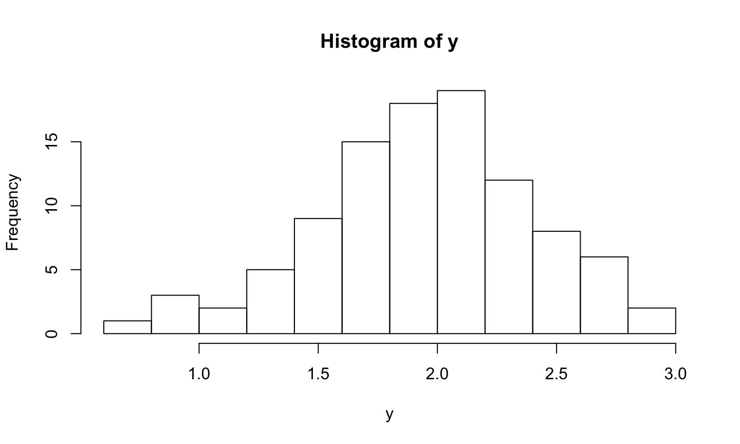
y = rnorm(n = 100, mean = 2, sd = 0.5) # N(2, 0.5)
```
Summary of x, y
Code (in a chunk):
```{r}
summary(x)
summary(y)
```
##    Min. 1st Qu.  Median    Mean 3rd Qu.    Max.
## -2.1435 -0.6226  0.1075  0.1305  0.8273  2.5863
##    Min. 1st Qu.  Median    Mean 3rd Qu.    Max.
##  0.7052  1.6464  1.9712  1.9492  2.2385  2.8509
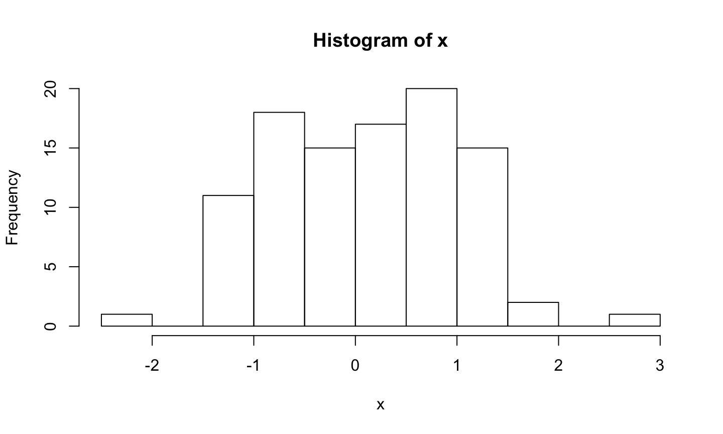
Histogram of x
Code (in a chunk):
```{r}
hist(x)
```
Histogram of y
Code (in a chunk):
```{r}
hist(y)
```
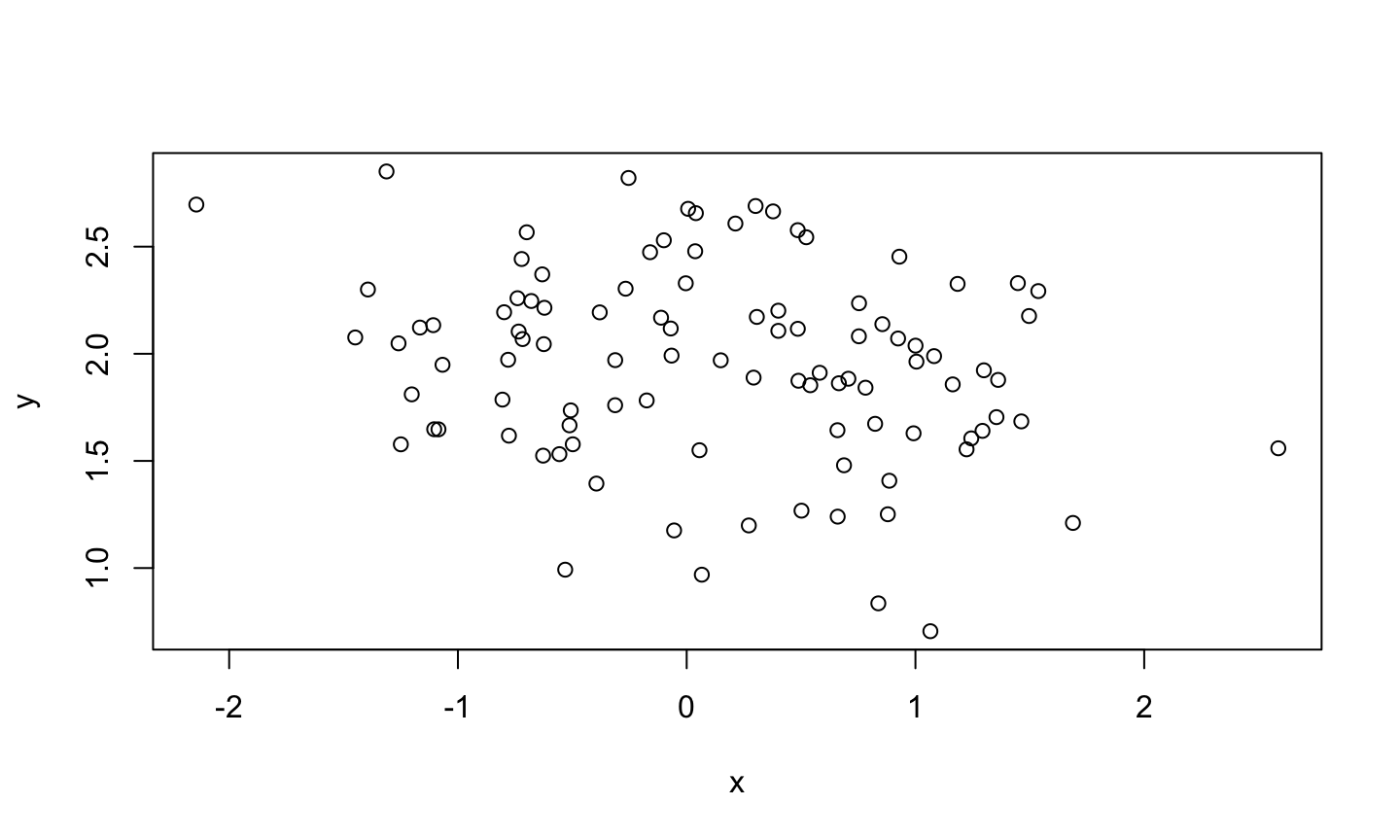
X vs. Y
Code (in a chunk):
```{r}
plot(x,y)
```
Embed a figure using “chunk” syntax
Code (in a chunk):
```{r rog, fig.cap="Rick's pic from Databrary"}
knitr::include_graphics("https://nyu.databrary.org/party/6/avatar")
```
Rick’s pic from Databrary
Embed a figure using HTML
Code (outside a chunk):
<img src="img/sleic.jpg" height=500px>
Height parameter (or, e.g. height=500px) is optional, but useful. Remember Markdown -> HTML.

Learn from my mistakes
- Don’t change your working directory…EVAH!
- Give R Markdown document “local” paths
- Projects (next week) make this MUCH easier
- Talk to R inside chunks; talk to RStudio outside chunks
- Save your R Markdown file often
Embed a YouTube video
HTML Code (outside a chunk–not talking to R)
<iframe width="420" height="315"
src="https://www.youtube.com/embed/9hUy9ePyo6Q"
frameborder="0" allowfullscreen>
</iframe>
- YouTube gives you code to cut and paste to ‘embed’ a video.
- Just copy and paste
Printing computed variables in your text
Code (in a chunk):
```{r}
summ.x = summary(x)
summ.y = summary(y)
names(summ.x) # Figure out variable names for indexing
```
## [1] "Min."    "1st Qu." "Median"  "Mean"    "3rd Qu."
## [6] "Max."
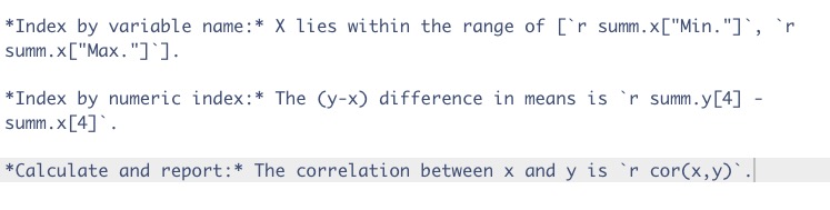
- Prefix inline code bits with “`r”
- Terminate inline code bits with single backtick “`”
- No more copying and pasting statistical results!
- Format numeric outputs with
sprintf() sprintf("%2.3f", 14.7666)gives 14.77- See
help("sprintf")
Index by variable name: X lies within the range of [-2.1434695, 2.5862562].
Index by numeric index: The (y-x) difference in means is 1.8187584.
Calculate and report: The correlation between x and y is -0.2262571.
Math equations
Markdown (not in a chunk–not talking to R) using LaTex syntax.
$$e=mc^{2}$$
\[e=mc^{2}\]
Doing real work with R Markdown
Use cases
- You want to give a talk based on your analysis
- You want to give a collaborator a report on your analysis in a format they prefer
- You don’t want to duplicate effort
Output options
- Document
- HTML
- Embedded or non-embedded figures
- MS Word
- HTML
- Presentation
- HTML (ioslides)
- HTML (Slidy)
- PDF (Beamer)
- Shiny (interactive document)
- Document
- Presentation (ioslides)
- A website!
All in your head(er)
- R Markdown documents have header text written in YAML
- YAML = YAML Ain’t Markup Language
---
title: "psy-525-rmarkdown-testbed"
author: "Rick Gilmore"
date: "2020-02-27 12:28:14"
output:
  html_document:
    self_contained: true
  word_document:
    fig_width: 5
    fig_height: 5
    fig_caption: false
    df_print: kable
  pdf_document: default
  ioslides_presentation: default
  powerpoint_presentation: default
---
Learn from my mistakes
- YAML syntax is specific
- Yes, the tabs and colons matter
- You can
have fun/waste a lot of time exploring YAML options
- OTOH, chunk options are super useful
echo=TRUEprints your R codeecho=FALSEruns but does not print your code;include=FALSEdoes also.eval=FALSEprevents a chunk from executing
‘Knitting’ vs. ‘Rendering’ your document
- Pressing the
knitbutton converts your document to the default format - That is, the first format after your
output:parameter - Pressing and holding the
knitbutton gives other options knitris an R package that R Markdown depends upon heavily
Rendering your document
In the console (not your R Markdown document):
> rmarkdown::render("testbed.Rmd")
Why render?
- Saves time when editing interactively
- Render, then switch to browser (alt-tab or command-tab)
- Refresh browser
- Give documents parameters, like which output(s) you want
In the console:
> rmarkdown::render("testbed.Rmd",
output_format = c("html_document", "word_document", "pdf_document"))
Makes copies in three different formats: testbed.html, testbed.docx, and testbed.pdf.
Other useful parameters for the rmarkdown::render() command
output_file = myslides.ioslides.htmloroutput_file = myslides.slidy.htmlto specify different output file targets.output_dir = reportsoroutput_dir = docxto direct output to a specific directory.- parameterized reports using
params:
In your header:
---
title: "psy-525-rmarkdown-testbed"
author: "Rick Gilmore"
date: "2020-02-27 12:28:14"
output:
  html_document: default
params:
  name: Joe
  quest: "to find the Holy Grail"
---
- Single words don’t require quotes; phrases with spaces do
In the console (for example):
> rmarkdown::render("testbed.Rmd", params=list(name="Francine"))
Some useful sets of YAML header parameters…
Make a self-contained HTML file that includes any plots you’ve made or graphics you’ve embedded. Great for sharing locally (i.e, as a document not over the web).
---
output:
  html_document:
    self_contained: true
---
Add a table of contents. toc_depth controls how “deep” into your header hierarchy the table of contents should go.
---
output:
  html_document:
    toc: true
    toc_depth: 2
---
Add toc_float: true to make the table of contents “float” to the side of your document.
---
output:
  html_document:
    toc: true
    toc_depth: 2
    toc_float: true
---
Add number_sections: true to make the table of contents automatically generate a hierarchical set of numbers–1.0, 1.2, 2.1, etc.–based on your header hierarchy. Remember, # is header 1, ## is header 2, etc.
---
output:
  html_document:
    toc: true
    toc_depth: 2
    toc_float: true
    number_sections: true
---
Include your code chunks (include = TRUE) but hide them until someone wants to see them by adding code_folding: hide to your YAML header.
---
output:
  html_document:
    toc: true
    toc_depth: 2
    toc_float: true
    number_sections: true
    code_folding: hide
---
Questions?
Your turn…
Next time
- RStudio projects
- Version control using git and GitHub
Resources
Software
This talk was produced on 2020-02-27 in RStudio using R Markdown. The code and materials used to generate the slides may be found at https://github.com/psu-psychology/psy-525-reproducible-research-2020. Information about the R Session that produced the code is as follows:
## R version 3.6.2 (2019-12-12)
## Platform: x86_64-apple-darwin15.6.0 (64-bit)
## Running under: macOS Mojave 10.14.6
##
## Matrix products: default
## BLAS:   /System/Library/Frameworks/Accelerate.framework/Versions/A/Frameworks/vecLib.framework/Versions/A/libBLAS.dylib
## LAPACK: /Library/Frameworks/R.framework/Versions/3.6/Resources/lib/libRlapack.dylib
##
## locale:
## [1] en_US.UTF-8/en_US.UTF-8/en_US.UTF-8/C/en_US.UTF-8/en_US.UTF-8
##
## attached base packages:
## [1] stats     graphics  grDevices utils     datasets
## [6] methods   base
##
## other attached packages:
##  [1] DiagrammeR_1.0.5 forcats_0.4.0    stringr_1.4.0
##  [4] dplyr_0.8.3      purrr_0.3.3      readr_1.3.1
##  [7] tidyr_1.0.0      tibble_2.1.3     ggplot2_3.2.1
## [10] tidyverse_1.3.0  seriation_1.2-8
##
## loaded via a namespace (and not attached):
##  [1] viridis_0.5.1      httr_1.4.1
##  [3] tufte_0.5          jsonlite_1.6
##  [5] viridisLite_0.3.0  foreach_1.4.8
##  [7] modelr_0.1.5       gtools_3.8.1
##  [9] assertthat_0.2.1   highr_0.8
## [11] cellranger_1.1.0   yaml_2.2.0
## [13] pillar_1.4.3       backports_1.1.5
## [15] lattice_0.20-38    glue_1.3.1
## [17] digest_0.6.23      RColorBrewer_1.1-2
## [19] rvest_0.3.5        colorspace_1.4-1
## [21] htmltools_0.4.0    pkgconfig_2.0.3
## [23] broom_0.5.3        haven_2.2.0
## [25] scales_1.1.0       gdata_2.18.0
## [27] farver_2.0.3       generics_0.0.2
## [29] withr_2.1.2        lazyeval_0.2.2
## [31] cli_2.0.1          magrittr_1.5
## [33] crayon_1.3.4       readxl_1.3.1
## [35] evaluate_0.14      fs_1.3.1
## [37] fansi_0.4.1        nlme_3.1-142
## [39] MASS_7.3-51.5      gplots_3.0.1.2
## [41] xml2_1.2.2         tools_3.6.2
## [43] registry_0.5-1     hms_0.5.3
## [45] lifecycle_0.1.0    munsell_0.5.0
## [47] reprex_0.3.0       cluster_2.1.0
## [49] packrat_0.5.0      compiler_3.6.2
## [51] caTools_1.18.0     rlang_0.4.4
## [53] grid_3.6.2         iterators_1.0.12
## [55] rstudioapi_0.10    visNetwork_2.0.9
## [57] htmlwidgets_1.5.1  labeling_0.3
## [59] bitops_1.0-6       rmarkdown_2.1
## [61] gtable_0.3.0       codetools_0.2-16
## [63] DBI_1.1.0          TSP_1.1-8
## [65] R6_2.4.1           gridExtra_2.3
## [67] lubridate_1.7.4    knitr_1.27
## [69] pwr_1.2-2          utf8_1.1.4
## [71] KernSmooth_2.23-16 dendextend_1.13.3
## [73] stringi_1.4.5      Rcpp_1.0.3
## [75] vctrs_0.2.2        gclus_1.3.2
## [77] dbplyr_1.4.2       tidyselect_1.0.0
## [79] xfun_0.12