2020-02-27 12:28:17
Preliminaries
Announcements
- Code for Her workshop on LaTex, 2020-02-26 6-8p, Paterno 103, Mann Assembly Room
- Data Science Community meeting 2020-02-28, 10a, Pattee Library Collaboration Commons
- Institute for Computational and Data Science (ICDS) events
- “The Data Deluge”, ICDS Symposium, March 16-17, 2020, NLI.
Today’s topics
- Some observations about GitHub use and R Markdown
- Simulation as a tool for reproducible and transparent science
- Visualization in R
- Advanced simulation
Observations
git/GitHub
- Add
.Rprojto your.gitignore. See Natalie’s stub. - You’re in charge of what goes where.
- Public repos are public, but no one knows what you’re doing unless you alert them.
- Pull first; edit second.
- Pull requests are when you edit my code and want me to “pull”/adopt it.
- If I’m a collaborator on the project with
writeprivileges, I don’t have to issue a pull request.
- If I’m a collaborator on the project with
R Markdown
- Ok to make multiple R Markdown files and link them
- Make sure to add spaces where they belong:
##Headervs.## Header - Comments! Add them. This is your record of what you did.
- Don’t forget you can hide things
- Label chunks
- Make chunks bite-sized
- Add comments in your code to explain what you’re doing
- Could someone else figure out what your code does?
Be a risk-taker; be your own professor
Simulation as a tool for reproducible and transparent science
- Why simulate
- What to simulate
- How to simulate
Why & what to simulate?
- Explore sample sizes, effect sizes, power
- Pre-plan/test, polish data-munging workflows
- Make hypotheses even more explicit
- Simulation == Pregistration on steroids
- ‘
X affects Y’ -> ‘Mean(X) > Mean(Y)’ - or ’Mean(X) >= 2*Mean(Y)’
- Simulate data analysis in advance
- Plan data visualizations in advance
- Avoid avoidable errors
- Plan your work, work your plan
- Super easy to run analyses when your data come in
How to simulate
- R functions
- R Markdown document(s)
Super-simple example
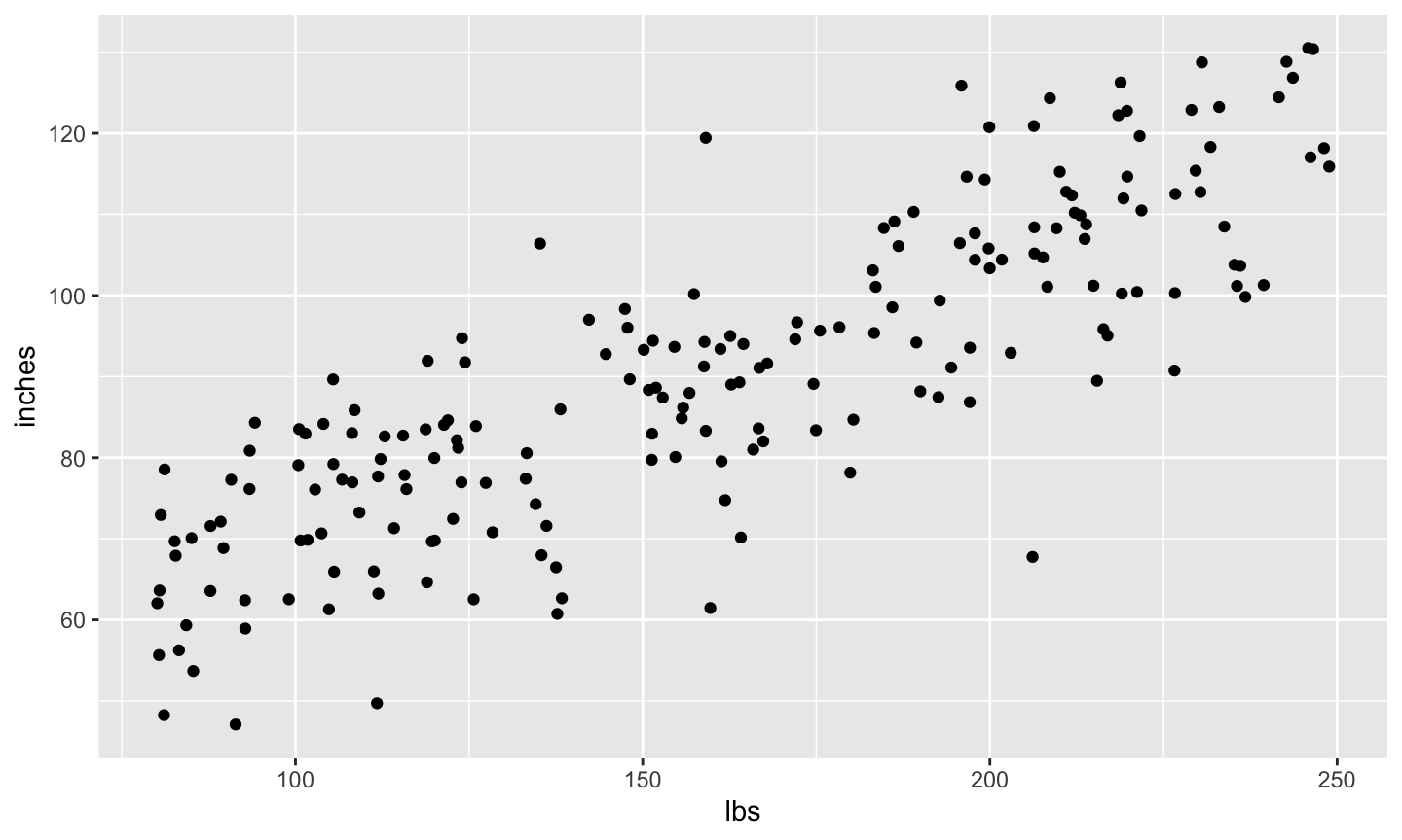
- Hypothesis 1: Height (inches) is correlated with weight (lbs)
# choose sample size
sample_n <- 200

# choose intercept and slope
beta0 <- 36   # inches
beta1 <- 0.33  # Rick's guess

# choose standard deviation for error
sigma <- 10 # Rick's guess
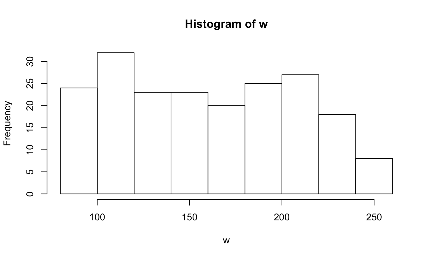
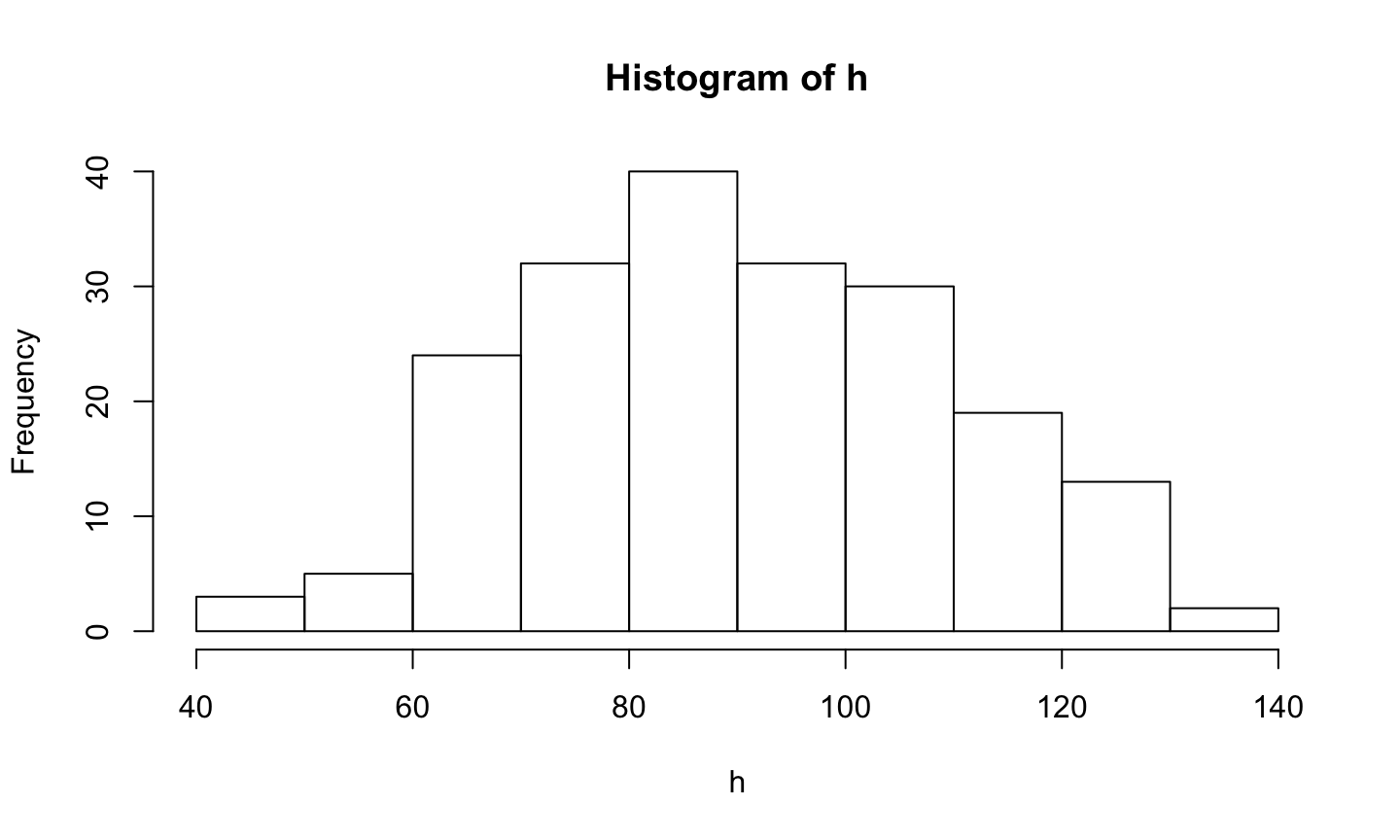
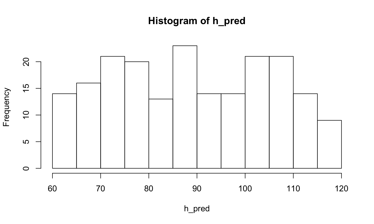
# random weights between 80 lbs and 250 lbs (uniform sampling)
w <- runif(n = sample_n, min = 80, max = 250)

h_pred <- rep(x = beta0, n = sample_n) + beta1 * w
h <- h_pred + rnorm(n = sample_n, mean = 0, sd = sigma)
library(ggplot2)
library(dplyr)

hist(w)
hist(h)
hist(h_pred)
# Put h and w into data frame for ggplot
height_weight <- data.frame(inches = h, lbs = w)

# Plot
scatter_1 <- ggplot2::ggplot(data = height_weight) +
  ggplot2::aes(x = lbs, y = inches) +
  ggplot2::geom_point()
scatter_1
Data pictures
- What should your data look like if your hypothesis is confirmed?
That’s synthesis, now analysis
- Remember Hypothesis 1: Height (inches) is correlated with weight (lbs)?
# Could use the raw data
# cor.test(x = w, y = h)
# Or, to use the values in the data frame, use with(...)

with(height_weight, cor.test(x = inches, y = lbs))
##
##  Pearson's product-moment correlation
##
## data:  inches and lbs
## t = 21.472, df = 198, p-value < 2.2e-16
## alternative hypothesis: true correlation is not equal to 0
## 95 percent confidence interval:
##  0.7892534 0.8737537
## sample estimates:
##       cor
## 0.8364064
Aside: extracting the statistics to make an interactive report
# Save output as a variable
cor_test_inches_lbs <- with(height_weight, cor.test(x = inches, y = lbs))

# What sort of beast is this?
mode(cor_test_inches_lbs)
## [1] "list"
# Aha, it's a list, this shows me all of the parts
unlist(cor_test_inches_lbs)
##                            statistic.t
##                     "21.4724896345742"
##                           parameter.df
##                                  "198"
##                                p.value
##                 "1.33502059642752e-53"
##                           estimate.cor
##                    "0.836406407472453"
##                 null.value.correlation
##                                    "0"
##                            alternative
##                            "two.sided"
##                                 method
## "Pearson's product-moment correlation"
##                              data.name
##                       "inches and lbs"
##                              conf.int1
##                    "0.789253416341088"
##                              conf.int2
##                    "0.873753662658475"
# Looks like the t value is the first element
cor_test_inches_lbs[[1]]
##        t
## 21.47249
The Pearson’s product-moment correlation between height and weight is 0.836, \(t\)(198)=21.472, \(p\)=0.00000, with a 95\(\%\) confidence interval of [0.789, 0.874].
I did some formatting using the sprintf() function to make the numbers look pretty. You may also find format() useful.
sprintf("%.3f", my.var) limits my.var to 3 decimal places; where sprintf("%2.3f", my.var) limits it to 2 digits to the left and 3 to the right.
Now back to analysis with our synthetic data
fit <- lm(formula = inches ~ lbs, data = height_weight)
summary(fit) # Use lm() command to fit formula
##
## Call:
## lm(formula = inches ~ lbs, data = height_weight)
##
## Residuals:
##     Min      1Q  Median      3Q     Max
## -37.103  -7.520   0.850   6.759  29.707
##
## Coefficients:
##             Estimate Std. Error t value Pr(>|t|)
## (Intercept) 38.58790    2.51316   15.35   <2e-16 ***
## lbs          0.32149    0.01497   21.47   <2e-16 ***
## ---
## Signif. codes:
## 0 '***' 0.001 '**' 0.01 '*' 0.05 '.' 0.1 ' ' 1
##
## Residual standard error: 10.44 on 198 degrees of freedom
## Multiple R-squared:  0.6996, Adjusted R-squared:  0.6981
## F-statistic: 461.1 on 1 and 198 DF,  p-value: < 2.2e-16
(ci <- confint(fit)) # confint() command fits confidence intervals
##                  2.5 %     97.5 %
## (Intercept) 33.6319130 43.5438961
## lbs          0.2919663  0.3510174
Surrounding (ci <- confint(fit)) in parentheses saves variable ci and prints it out.
How’d we do?
| Parameter | Actual | Low Estimate | High Estimate |
|---|---|---|---|
| \(\beta0\) | 36 | 33.631913 | 43.5438961 |
| \(\beta1\) | 0.33 | 0.2919663 | 0.3510174 |
# random weights between 80 lbs and 250 lbs (uniform sampling)
w <- runif(n = sample_n, min = 80, max = 250)

h_pred <- rep(x = beta0, n = sample_n) + beta1 * w
h <- h_pred + rnorm(n = sample_n, mean = 0, sd = sigma)
height_weight <- data.frame(inches = h, lbs = w)

fit <- lm(formula = inches ~ lbs, data = height_weight)
summary(fit)
##
## Call:
## lm(formula = inches ~ lbs, data = height_weight)
##
## Residuals:
##      Min       1Q   Median       3Q      Max
## -24.8229  -7.5843   0.0817   6.1271  29.6438
##
## Coefficients:
##             Estimate Std. Error t value Pr(>|t|)
## (Intercept) 34.88577    2.48984   14.01   <2e-16 ***
## lbs          0.33834    0.01465   23.09   <2e-16 ***
## ---
## Signif. codes:
## 0 '***' 0.001 '**' 0.01 '*' 0.05 '.' 0.1 ' ' 1
##
## Residual standard error: 9.794 on 198 degrees of freedom
## Multiple R-squared:  0.7293, Adjusted R-squared:  0.7279
## F-statistic: 533.4 on 1 and 198 DF,  p-value: < 2.2e-16
(ci <- confint(fit)) # saves in variable ci and prints
##                  2.5 %     97.5 %
## (Intercept) 29.9757671 39.7957796
## lbs          0.3094516  0.3672307
| Parameter | Actual | Low Estimate | High Estimate |
|---|---|---|---|
| \(\beta0\) | 36 | 29.9757671 | 39.7957796 |
| \(\beta1\) | 0.33 | 0.3094516 | 0.3672307 |
Simulation of neural data
- Critical review: Welvaert, M., & Rosseel, Y. (2014). A Review of fMRI Simulation Studies. PLOS ONE, 9(7), e101953. https://doi.org/10.1371/journal.pone.0101953.
- Welvaert, M., Durnez, J., Moerkerke, B., Berdoolaege, G. & Rosseel, Y. (2011). neuRosim: An R Package for Generating fMRI Data. Journal of Statistical Software, 44(10). Retrieved from https://www.jstatsoft.org/article/view/v044i10
- AFNI’s AlphaSim, https://afni.nimh.nih.gov/pub/dist/doc/program_help/AlphaSim.html
- Simulating EEG data
- https://github.com/lrkrol/SEREEGA
eegkitR package haseegsimfunction
Visualization in R
Plot first, analyze last
- Why?
- Mike Meyer told me so
- Less biased
- Easier to be transparent and reproducible
- Want/need to plot eventually anyway
- If a picture’s worth a thousand words…
- How?
Things I feel strongly about
- Plot all of your data
- Every response, condition, participant
- What do the plots tell you?
- Do your plots match your prior ‘data picture’?
How
- Base graphics
plot(x,y)hist(x),coplot()
ggplot2- Grammar of graphics
Base graphics
- Try it, maybe you’ll like it
plot()takes many types of input- So does
summary() - A little harder to customize
Data visualization with ggplot2
- The
ggrefers to the Grammar of Graphics
Wilkinson, L., Wills, D., Rope, D., Norton, A., & Dubbs, R. (2005). The Grammar of Graphics (Statistics and Computing) (2nd edition.). Springer. Retrieved from https://www.amazon.com/Grammar-Graphics-Statistics-Computing/dp/0387245448
ggplot2is the package;ggplot()is the function call- Data can be continuous, ordinal, or nominal
- Graphs map data \(\rightarrow\) visual elements (aesthetics)
- {height, weight, gender, rt} \(\rightarrow\) {x, y, color, shape, line type, row, column}
- ‘Add’ layers to our plot using the
+operator
Learning ggplot
- Wickham, H. & Grolemund, G. (2017). R for Data Science. O’Reilly. http://r4ds.had.co.nz/
Let’s walk through the data visualiation chapter
Other ggplot2 resources
- ggplot2 3.2.1 documentation: http://docs.ggplot2.org/current/
- Wickham, H. (2010). ggplot2: Elegant Graphics for Data Analysis (Use R!) http://ggplot2.org/book/
- Chang, Winston (2013). R Graphics Cookbook. O’Reilly.
- Kieran Healy’s workshop at RStudio::Conf 2020
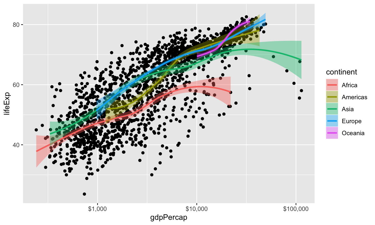
Example from K. Healy talk
## `geom_smooth()` using method = 'loess' and formula 'y ~ x'
Advanced simulation
Advanced simulation
- Putting code into a function
- A factorial design?
Let’s make it a function
- Functions help automate routines
- Parts of a function:
- Input parameters
- Defaults or not
- Output(s)
- Input parameters
my_function_name <- function(my_param1, my_param2 = "cool")
# define global constants from prior simulation
sample_n = 200
beta0 = 36
beta1 = .33
sigma = 10
min_x = 80
max_x = 250
height_weight_sim <- function(sample_n = 200, beta0 = 36, beta1 = .33, sigma = 10, min_x = 80, max_x = 250) {
  # Calculates correlation, intercept, slope estimates for
  # linear relation between two variables

  # Args:
  #   sample_n: Number of sample poings, default is 200
  #   beta0: Intercept, default is 36 (inches)
  #   beta1: Slope, default is .33
  #   sigma: Standard deviation of error
  #   min_x: Minimum value for x (weight in lbs)
  #   max_x: Maximum value for x (weight in lbs)
  #
  # Returns:
  #   Named array with values
  #   beta0
  #   beta1
  #   beta0.lo: 2.5% quantile for intercept
  #   beta0.hi  97.5% quantile for intercept
  #   beta1.lo  2.5% quantile for slope
  #   beta1.hi  97.5% quantile for slope

  w <- runif(n = sample_n, min = min_x, max = max_x)

  h_pred <- rep(x = beta0, n = sample_n) + beta1 * w
  h <- h_pred + rnorm(n = sample_n, mean = 0, sd = sigma)
  height.weight <- data.frame(inches = h, lbs = w)

  fit <- lm(formula = inches ~ lbs, data = height.weight)
  ci <- confint(fit)

  # Create output vector with named values
  (results <- c("beta0" = beta0,
    "beta1"= beta1,
    "beta0.lo" = ci[1,1],
    "beta0.hi" = ci[1,2],
    "beta1.lo" = ci[2,1],
    "beta1.hi" = ci[2,2]))
}
# Defaults only
height_weight_sim()
##      beta0      beta1   beta0.lo   beta0.hi   beta1.lo
## 36.0000000  0.3300000 30.6497291 40.0010555  0.3066327
##   beta1.hi
##  0.3610621
# Larger sample size
height_weight_sim(sample_n = 500)
##      beta0      beta1   beta0.lo   beta0.hi   beta1.lo
## 36.0000000  0.3300000 33.3918123 39.6015099  0.3081033
##   beta1.hi
##  0.3444201
Doing a series of simulations
- Goal: run our function a number of times, collect the results
n_simulations = 100
n_vars = 6 # variables height_weight_sim() outputs

# initialize output array
height_weight_sim_data <- array(0, dim=c(n_simulations, n_vars))

# Repeat height_weight_sim() n_simulations times
for (i in 1:n_simulations) {
  height_weight_sim_data[i,] <- height_weight_sim()
  }
# Easier to make simulation data a data frame
ht_wt_sims <- as.data.frame(height_weight_sim_data)
# rename variables to be more easily read
names(ht_wt_sims) <- c("beta0", "beta1",
"beta0.lo", "beta0.hi",
"beta1.lo", "beta1.hi")
# Add a variable to index the simulation number
ht_wt_sims$sim_num <- 1:n_simulations
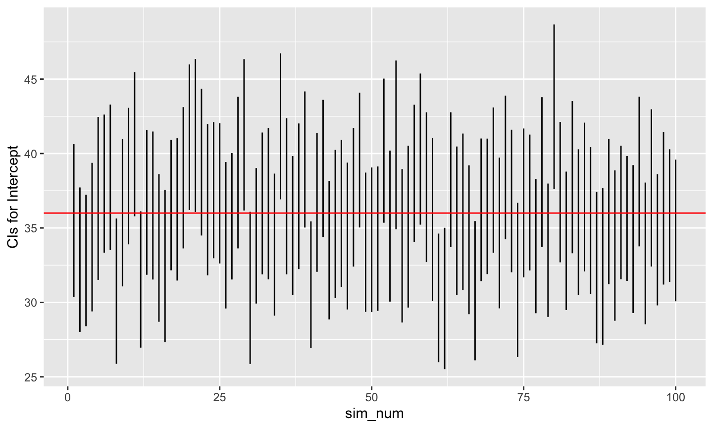
# Plot beta0 min and max (now called V3, V4)
ggplot(data = ht_wt_sims) +
aes(x = sim_num) +
geom_linerange(mapping = aes(ymin = beta0.lo,
ymax = beta0.hi)) +
ylab("CIs for Intercept") +
geom_hline(yintercept = beta0, color = "red")
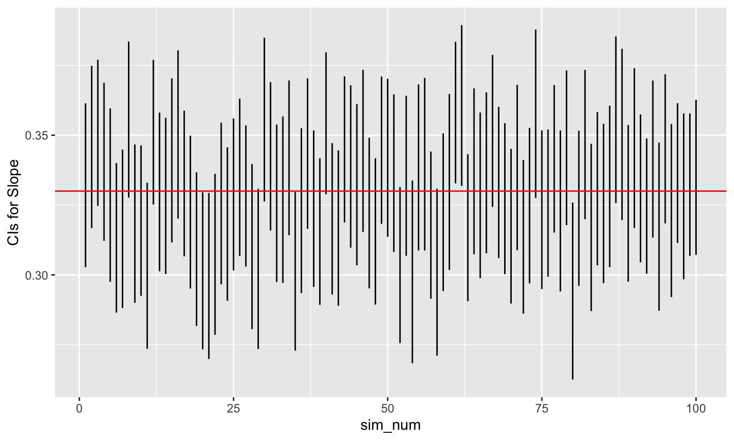
# Plot beta1 min and max (now called V5, V6)
ggplot(data = ht_wt_sims) +
  aes(x = sim_num) +
  geom_linerange(mapping = aes(ymin = beta1.lo,
                                ymax = beta1.hi)) +
  ylab("CIs for Slope") +
  geom_hline(yintercept = beta1, color = "red")
How about a factorial design?
- Dependent variable: RT
- Independent variables
- Fixed
- Symbol type: {letter, number}
- Random
- Subject mean RT
- Fixed
- Hypothesis:
- RT to detect numbers is bigger than for letters (by 50 ms)
- There is no order effect
- Rick wishes he’d found this first: https://www.r-bloggers.com/design-of-experiments-%E2%80%93-full-factorial-designs/
# Simulation parameters
n_subs = 30
trials_per_cond = 100
letters_numbers_rt_diff = 50 # ms
rt_mean_across_subs = 350
sigma = 50
cond_labels = c("letter", "number")
cond_rts <- c("letter" = 0, "number" = letters_numbers_rt_diff)
stim_types <- factor(x = rep(x = c(1,2),
trials_per_cond),
labels = cond_labels)
#sample(factor(x=rep(c("letter", "number"), 100)), 200)
random_stim_types <- sample(stim_types, trials_per_cond*length(cond_labels))
mean_sub_rt <- rnorm(n = 1, mean = rt_mean_across_subs, sd = sigma)
trial_rt <- array(0, dim = length(random_stim_types))
# Generate RTs based on trial, condition
for (t in 1:length(random_stim_types)) {
trial_rt[t] <- mean_sub_rt + cond_rts[random_stim_types[t]] +
rnorm(n = 1, mean = 0, sd = sigma)
}
# Make data frame
letter_number_df <- data.frame(trial = 1:length(random_stim_types),
stim = random_stim_types,
rt = trial_rt)
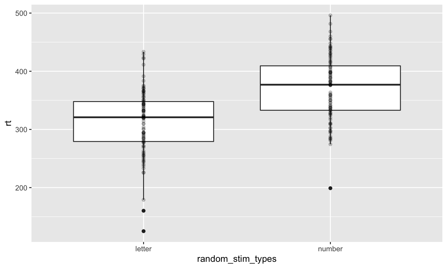
letter_number_df %>%
ggplot(.) +
aes(x = random_stim_types, y = rt) +
geom_boxplot() +
geom_point(alpha = .2)
Put this in a function
simulate_sub_rt <- function(trials_per_cond = 100,
                            letters_numbers_rt_diff = 50,
                            rt_mean_across_subs = 350,
                            sigma = 50) {

  cond_rts <- c("letter" = 0,
                "number" = letters_numbers_rt_diff)
  stim_types <- factor(x = rep(x = c(1,2),
                               trials_per_cond),
                       labels = c("letter", "number"))
  random_stim_types <- sample(stim_types, 2*trials_per_cond)

  mean_sub_rt <- rnorm(n = 1,
                       mean = rt_mean_across_subs,
                       sd = sigma)
  trial_rt <- array(0, dim = length(random_stim_types))

  # Generate RTs based on trial, condition
  for (t in 1:length(random_stim_types)) {
    trial_rt[t] <- mean_sub_rt + cond_rts[random_stim_types[t]] +
      rnorm(n = 1, mean = 0, sd = sigma)
    }

  # Make data frame
  letter.number.df <- data.frame(trial = 1:length(random_stim_types),
                                 stim = random_stim_types,
                                 rt = trial_rt)
}
Create code to a set of participants and create one merged data frame
make_sub_rt_df <- function(sub.id) {
  sub_rt_df <- simulate_sub_rt()
  sub_rt_df$sub.id <- sub.id
  sub_rt_df
}

# Use lapply to make separate data frames for all subs
sub_rt_df_list <- lapply(1:n_subs, make_sub_rt_df)

# Use Reduce() with the merge function to make one big file
sub_rt_df_merged <- Reduce(function(x, y) merge(x, y, all=TRUE), sub_rt_df_list)
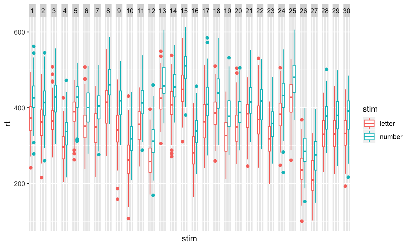
Now, want to see what we have?
ggplot(data = sub_rt_df_merged) +
  aes(x=stim, y=rt, color=stim) +
  geom_boxplot() +
  facet_grid(facets = . ~ as.factor(sub.id)) +
  theme(axis.text.x.bottom = element_blank(),
        axis.ticks.x.bottom = element_blank())
And, just for fun
library(lme4)
fit1 <- lmer(formula = rt ~ stim + (1|sub.id), data = sub_rt_df_merged)
summary(fit1)
## Linear mixed model fit by REML ['lmerMod']
## Formula: rt ~ stim + (1 | sub.id)
##    Data: sub_rt_df_merged
##
## REML criterion at convergence: 64209.2
##
## Scaled residuals:
##     Min      1Q  Median      3Q     Max
## -4.0626 -0.6703  0.0011  0.6620  3.3775
##
## Random effects:
##  Groups   Name        Variance Std.Dev.
##  sub.id   (Intercept) 3081     55.51
##  Residual             2535     50.35
## Number of obs: 6000, groups:  sub.id, 30
##
## Fixed effects:
##             Estimate Std. Error t value
## (Intercept)   347.26      10.18   34.13
## stimnumber     50.62       1.30   38.94
##
## Correlation of Fixed Effects:
##            (Intr)
## stimnumber -0.064
Or
fit2 <- aov(formula = rt ~ stim + Error(as.factor(sub.id)), data = sub_rt_df_merged)
summary(fit2)
##
## Error: as.factor(sub.id)
##           Df   Sum Sq Mean Sq F value Pr(>F)
## Residuals 29 17943263  618733
##
## Error: Within
##             Df   Sum Sq Mean Sq F value Pr(>F)
## stim         1  3843699 3843699    1516 <2e-16 ***
## Residuals 5969 15131695    2535
## ---
## Signif. codes:
## 0 '***' 0.001 '**' 0.01 '*' 0.05 '.' 0.1 ' ' 1
Next time
- Doing other useful things with R and R Markdown
Resources
Software
This talk was produced on 2020-02-27 in RStudio using R Markdown. The code and materials used to generate the slides may be found at https://github.com/psu-psychology/psy-525-reproducible-research-2020. Information about the R Session that produced the code is as follows:
## R version 3.6.2 (2019-12-12)
## Platform: x86_64-apple-darwin15.6.0 (64-bit)
## Running under: macOS Mojave 10.14.6
##
## Matrix products: default
## BLAS:   /System/Library/Frameworks/Accelerate.framework/Versions/A/Frameworks/vecLib.framework/Versions/A/libBLAS.dylib
## LAPACK: /Library/Frameworks/R.framework/Versions/3.6/Resources/lib/libRlapack.dylib
##
## locale:
## [1] en_US.UTF-8/en_US.UTF-8/en_US.UTF-8/C/en_US.UTF-8/en_US.UTF-8
##
## attached base packages:
## [1] stats     graphics  grDevices utils     datasets
## [6] methods   base
##
## other attached packages:
## [1] lme4_1.1-21     Matrix_1.2-18   gapminder_0.3.0
## [4] dplyr_0.8.4     ggplot2_3.2.1
##
## loaded via a namespace (and not attached):
##  [1] Rcpp_1.0.3         nloptr_1.2.1
##  [3] plyr_1.8.5         pillar_1.4.3
##  [5] compiler_3.6.2     tools_3.6.2
##  [7] boot_1.3-23        digest_0.6.25
##  [9] packrat_0.5.0      nlme_3.1-142
## [11] lattice_0.20-38    evaluate_0.14
## [13] lifecycle_0.1.0    tibble_2.1.3
## [15] gtable_0.3.0       pkgconfig_2.0.3
## [17] rlang_0.4.4        yaml_2.2.1
## [19] xfun_0.12          withr_2.1.2
## [21] stringr_1.4.0      knitr_1.28
## [23] grid_3.6.2         tidyselect_1.0.0
## [25] tufte_0.5          glue_1.3.1
## [27] R6_2.4.1           databraryapi_0.1.9
## [29] rmarkdown_2.1      minqa_1.2.4
## [31] purrr_0.3.3        farver_2.0.3
## [33] reshape2_1.4.3     magrittr_1.5
## [35] MASS_7.3-51.5      splines_3.6.2
## [37] scales_1.1.0       htmltools_0.4.0
## [39] assertthat_0.2.1   colorspace_1.4-1
## [41] labeling_0.3       stringi_1.4.6
## [43] lazyeval_0.2.2     munsell_0.5.0
## [45] crayon_1.3.4