2018-01-29 The retinal image

# 2018-01-29 The retinal image
## PSY 525.001 • Vision Science • 2018 Spring
### Rick Gilmore
### 2018-01-29 08:21:13

---

# Today's topics

--
## The retinal image

--
## Discuss Fourier analysis, esp. Campbell & Robson 1968.

---
class: center, middle, inverse

# The retinal image

---
class: center, middle

# Human retina

<http://webvision.med.utah.edu/>
---

<http://webvision.med.utah.edu/>

---
class: center, middle

## Ganglion cell response properties differ across cells

## Individual response function of stimulus location, size

## On- and off-center cells

## Receptive fields have *center-surround* structure, due to *lateral inhibition*

---
class: center, middle

<p><a href="https://commons.wikimedia.org/wiki/File:Receptive_field.png#/media/File:Receptive_field.png"><img src="https://upload.wikimedia.org/wikipedia/commons/1/16/Receptive_field.png" alt="Receptive field.png" height=450px></a><br>By original uploaded to en by <a href="//commons.wikimedia.org/wiki/User:Delldot" title="User:Delldot">user:delldot</a>, modified by <a href="//commons.wikimedia.org/w/index.php?title=User:Xoneca&amp;action=edit&amp;redlink=1" class="new" title="User:Xoneca (page does not exist)">Xoneca</a> - <span class="int-own-work" lang="en" xml:lang="en">Own work</span>, Public Domain, <a href="https://commons.wikimedia.org/w/index.php?curid=5714283">Link</a></p>

---
class: center, middle

photoreceptors -> horizontal cells; photoreceptors + horizontal cells -> bipolar cells; bipolar cells -> amacrine + ganglion cells; bipolar + amacrine -> ganglion cells

---
class: center, middle

## Retina -> Lateral Geniculate Nucleus (LGN) of thalamus

---
class: center, middle

---
class: center, middle

## Parvocellular (small cell) and magnocellular (large cell) layers

## Inputs from ipsilateral (2, 3, 5) and contralateral (1, 4, 6) eye separate by layer

## Retinal geometry aligned

---
class: middle

# Magno vs. parvo LGN cells

| Characteristic       | Parvo | Magno |
|----------------------|-------|-------|
| Color sensitivity    | High  | Low   |
| Contrast sensitivity | Low   | High  |
| Spatial resolution   | High  | Low   |
| Temporal resolution  | Slow  | Fast  |
| Receptive field size | Small | Large |

### Palmer Table 4.1.1

---
class: center, middle

# Visual cortex

Striate cortex (stria of Gennari), V1, (Brodmann) area 17

---
class: center, middle

---
class: center, middle

---
class: center, middle

## Mapping visual cortex by hand

---
class: center, middle
## Center-surround cells rare & rarity surprising

## Simple cells, complex cells, & hypercomplex cells were elongated

---
class: center, middle

## Simple cells

---
class: center, middle

## Orientation (angular) selectivity

---
class: center, middle
## Complex cells

### Nonlinear, motion sensitive, position invariance, spatially extended

---
class: center, middle
## Hypercomplex (end-stopped) cells

---
class: center, middle

## Cortical magnification

---
class: center, middle

<http://cns.bu.edu/~arash/animation.gif>

---
class: center, middle

## Retinotopy

---
class: center, middle

## Expanding ring/annulus

---
class: center, middle

## Rotating wedge

---
class: center, middle

---
class: center, middle

Zhuang, J., Ng, L., Williams, D., Valley, M., Li, Y., Garrett, M., & Waters, J. (2017). An extended retinotopic map of mouse cortex. eLife, 6. Retrieved from http://dx.doi.org/10.7554/eLife.18372

---
class: center, middle

## Ocular dominance

---
class: center, middle

## Cortical hypercolumn

---
class: center

# Aspects of the retinal-> V1 image

## Topographic, but non-uniform

## Functionally segregated (on/off center, wavelength, eye of origin)

---
class: center, middle, inverse

# Spatial frequency analysis

---
class: middle, center

# But first a bit about images as arrays of numbers

---
class: middle

```r
pix_per_img <- 100
x <- (1:pix_per_img)/pix_per_img  # Make x on (0,1]
cyc_per_img <- 2                  # spatial frequency f
phase <- 0
one_row <- sin(2*pi*cyc_per_img*x + phase)
plot(one_row)
```

![](2018-01-29-retinal-image_files/figure-html/unnamed-chunk-1-1.png)

---
class: middle

```r
sin_array <- array(rep(one_row, pix_per_img), 
                   dim = c(pix_per_img, pix_per_img))
sin_img <- as.cimg(sin_array) # Nice image format from package imager
plot(sin_img)
```

![](2018-01-29-retinal-image_files/figure-html/unnamed-chunk-2-1.png)

---
class: middle

```r
vertical_grating <- function(pix_per_img=100, cyc_per_img=1, phase=0){
  x <- (1:pix_per_img)/pix_per_img 
  one_row <- (sin(2*pi*cyc_per_img*x + phase)+1)*0.5 # Scale to [0,1]
  as.cimg(array(rep(one_row, pix_per_img),
                   dim = c(pix_per_img, pix_per_img)))
}
```

---
class: middle

```r
vg_100 <- vertical_grating(cyc_per_img = 5)
plot(vg_100, rescale = FALSE)
```

![](2018-01-29-retinal-image_files/figure-html/unnamed-chunk-4-1.png)

---
class: middle

```r
vg_50 <- vg_100*0.5
plot(vg_50, rescale = FALSE)
```

![](2018-01-29-retinal-image_files/figure-html/vg_50-1.png)

---
class: middle

```r
vg_25 <- vg_100*.25
plot(vg_25, rescale = FALSE)
```

![](2018-01-29-retinal-image_files/figure-html/vg_25-1.png)

---
# Under the hood

- Value at each `$x,y$` pixel is a number `$[0,1]$` (for grayscale)
- `plot` scales that to [0,255] (dark to light)
- [0,255] has 256 levels, `$2^8=256$`, so this is '8-bit grayscale'
- 8-bit color has 3 numbers at each pixel, `$(r,g,b)$`, one each for the **r**ed, **g**reen, and **b**lue values.

---
class: middle, center

# Synthesizing images from sums of gratings

## Every ~~periodic~~ pattern consists of an infinite sum of gratings of different spatial frequency, amplitude, phase, and orientation

---
class: middle

```r
grating <- function(pix_per_img=100, cyc_per_img=1, 
                    phase=0, vertical=TRUE){
  x <- (1:pix_per_img)/pix_per_img 
  one_row <- (sin(2*pi*cyc_per_img*x + phase)+1)*0.5 # Scale to [0,1]
  many_rows <- array(rep(one_row, pix_per_img),
                     dim = c(pix_per_img, pix_per_img))
  if (vertical)
    as.cimg(many_rows)
  else as.cimg(t(many_rows)) # transpose (rotate 90 deg)
}
```

---

```r
plot(grating(cyc_per_img = 10))
```

![](2018-01-29-retinal-image_files/figure-html/unnamed-chunk-6-1.png)

---
class: middle

```r
plot(grating(cyc_per_img = 10, vertical=FALSE))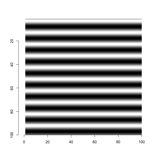
```

![](2018-01-29-retinal-image_files/figure-html/unnamed-chunk-7-1.png)

---
class: middle

```r
g_vert <- grating(cyc_per_img = 10, vertical = TRUE)
g_horiz <- grating(cyc_per_img = 10, vertical = FALSE)
g_sum <- g_vert + g_horiz
plot(g_sum)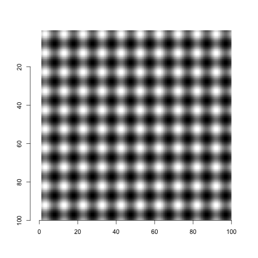
```

![](2018-01-29-retinal-image_files/figure-html/unnamed-chunk-8-1.png)

---
class: middle

# Synthesizing a square wave

```r
f <- 2 # Cycles per image
f1 <- grating(cyc_per_img = f)
f3 <- grating(cyc_per_img = 3*f)*(1/3)
f5 <- grating(cyc_per_img = 5*f)*(1/5)
f7 <- grating(cyc_per_img = 7*f)*(1/7)
f9 <- grating(cyc_per_img = 9*f)*(1/9)
```

---
class: middle

```r
plot(f1)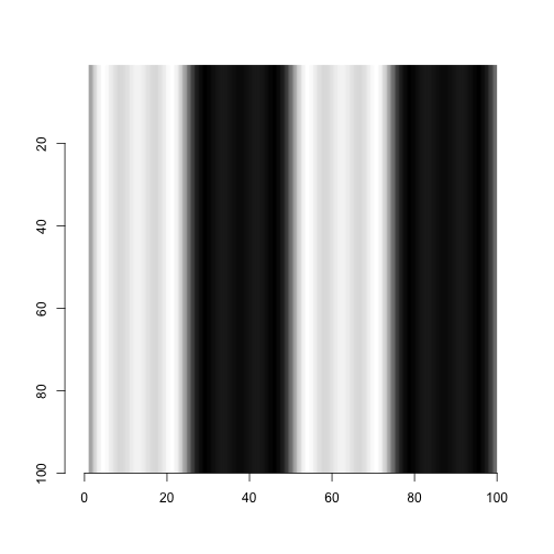
```

![](2018-01-29-retinal-image_files/figure-html/unnamed-chunk-10-1.png)

---
class: middle

```r
plot(f1+f3)
```

![](2018-01-29-retinal-image_files/figure-html/unnamed-chunk-11-1.png)

---
class: middle

```r
plot(f1+f3+f5)
```

![](2018-01-29-retinal-image_files/figure-html/unnamed-chunk-12-1.png)

---
class: middle

```r
plot(f1+f3+f5+f7)
```

![](2018-01-29-retinal-image_files/figure-html/unnamed-chunk-13-1.png)

---
class: middle

```r
plot(f1+f3+f5+f7+f9)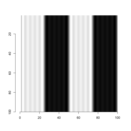
```

![](2018-01-29-retinal-image_files/figure-html/unnamed-chunk-14-1.png)

---
class: middle

# Why this works

```r
plot(f1[,1,1,1], ylim = c(0,1))
```

![](2018-01-29-retinal-image_files/figure-html/unnamed-chunk-15-1.png)

---
class: middle

```r
plot(f1[,1,1,1]+f3[,1,1,1])
```

![](2018-01-29-retinal-image_files/figure-html/unnamed-chunk-16-1.png)

---
class: middle

```r
plot(f1[,1,1,1]+f3[,1,1,1]+f5[,1,1,1])
```

![](2018-01-29-retinal-image_files/figure-html/unnamed-chunk-17-1.png)

---
class: middle

```r
plot(f1[,1,1,1]+f3[,1,1,1]+f5[,1,1,1]+f7[,1,1,1])
```

![](2018-01-29-retinal-image_files/figure-html/unnamed-chunk-18-1.png)

---
class: center, middle

# That's (Fourier) *synthesis*

component_1 + component_2 +...+ component_n = image

---
class: center, middle

---
class: center, middle
# Fourier *analysis* goes in reverse

image = component_1 + component_2 +...+ component_n

---
class: center, middle

<p><a href="https://commons.wikimedia.org/wiki/File:Fourier_transform_time_and_frequency_domains_(small).gif#/media/File:Fourier_transform_time_and_frequency_domains_(small).gif"><img src="https://upload.wikimedia.org/wikipedia/commons/7/72/Fourier_transform_time_and_frequency_domains_%28small%29.gif" alt="Fourier transform time and frequency domains (small).gif"></a><br>By <a href="//commons.wikimedia.org/wiki/User:LucasVB" title="User:LucasVB">Lucas V. Barbosa</a> - <span class="int-own-work" lang="en">Own work</span>, Public Domain, <a href="https://commons.wikimedia.org/w/index.php?curid=24830373">Link</a></p>

---
class: center, middle

## Why is Fourier analysis useful and important for vision science?

## Why is it useful and important for other areas of psychological or neural science?

---
class: center, middle, inverse

# Break time

---
class: center, middle, inverse

# Discussion of Campbell, F. W., & Robson, J. G. (1968).

---
# Key terms & parameters
- Contrast sensitivity vs. contrast threshold
- Contrast sensitivity function
- Sine, square, rectangular, saw tooth gratings
- Fourier components
- Luminance (in `$cd/m^2$`)
- Spatial frequency (in `$cyc/deg$`) vs. spatial period ($deg/cyc$)
- Temporal frequency (in `$c/s$`)
- Duty cycle `$(0,1]$`
- Size of image (in deg)
- Viewing distance
- Fundamental frequency

---
# Contrast sensitivity

- sensitivity = 1/threshold
- low threshold -> high sensitivity & *vice versa*

---
class: center, middle
# Spatial frequency

Rules of thumb (~$1-2^{\circ}$), vertical fist (~$5^{\circ}$), horizontal fist ($10^{\circ}$)

---
class: center, middle

Three vertical sine wave gratings at low, medium, and high spatial frequency

---
# Fourier components

- **Sine wave**: `$$\frac{4m}{\pi}sin(\frac{2\pi x}{X})$$`
where `$X$` is the period, `$\frac{x}{cycle}$`, or `$\frac{1}{frequency}$` and `$m$` is the contrast, `$\frac{L_{max}-L_{min}}{2\bar L}$`
- There are many measures of contrast, see <https://en.wikipedia.org/wiki/Contrast_(vision)>
- **Square wave**: `$$\frac{4m}{\pi}[\frac{1}{1}sin(1\frac{2\pi x}{X})+\frac{1}{3}sin(3\frac{2\pi x}{X})+\frac{1}{5}sin(5\frac{2\pi x}{X})+...]$$`

---
class: middle, center

# Duty cycle

---
# Questions

- What psychophysical method was used?
- How were thresholds estimated?
- Why might a larger aperture yield higher sensitivity (lower threshold)?
- What spatial frequency yields the highest sensitivity?

---
# Evaluating Campbell & Robson (1968) claims

1. The contrast thresholds of a variety of grating patterns have been
measured over a wide range of spatial frequencies.
2. Contrast thresholds for the detection of gratings whose luminance
profiles are sine, square, rectangular or saw-tooth waves can be simply
related using Fourier theory.
3. Over a wide range of spatial frequencies the contrast threshold of a
grating is determined only by the amplitude of the fundamental Fourier
component of its wave form.
4. Gratings of complex wave form cannot be distinguished from sinewave
gratings until their contrast has been raised to a level at which the
higher harmonic components reach their independent threshold.
5. These findings can be explained by the existence within the nervous
system of linearly operating independent mechanisms selectively sensitive
to limited ranges of spatial frequencies.

---
# The bigger picture

- Is V1 detecting oriented lines or spatial frequency patterns?
- [**Gabor patches**](https://www.cogsci.nl/pages/gabor-generator) combine a grating and a Gaussian envelope

---
<img src="http://www.extreme-eye-exercise.com/images/3.jpg">

Gabor patches as models of V1 simple cells?

---
class: middle, center

Real component

`$$g(x,y;\lambda, \theta, \psi, \sigma, \gamma)=exp(-\frac{x'^2+\gamma^2y'^2}{2\sigma^2})cos(2\pi\frac{x'}{\lambda} + \psi)$$`
Imaginary component

`$$g(x,y;\lambda, \theta, \psi, \sigma, \gamma)=exp(-\frac{x'^2+\gamma^2y'^2}{2\sigma^2})sin(2\pi\frac{x'}{\lambda} + \psi)$$`

with `$x'=xcos(\theta)+ysin(\theta)$` and `$y'=-x sin(\theta) + ycos(\theta)$`

---
class: center, middle

---
class: center, middle

|Snellen Metric | Snellen Imperial | MAR | logMAR | Decimal | cyc/deg |
|--------------|------------------|-----|--------|---------|--------- |
| 6/60	       | 20/200	          | 10	| 1.0	   | 0.10    | 3        |
| 6/48	       | 20/160	          | 8.0	| 0.9	   | 0.13    |          |
| 6/38	       | 20/125	          | 6.3	| 0.8	   | 0.16    | 4.76
| 6/30	       | 20/100	          | 5.0	| 0.7	   | 0.20    ||
| 6/24	       | 20/80	          | 4.0	| 0.6	   | 0.25    ||
| 6/19	       | 20/60		        | 3.2	| 0.5	   | 0.32    | 9.375    |
| 6/15	       | 20/50		        | 2.5	| 0.4    | 0.40    ||
| 6/12	       | 20/40		        | 2.0	| 0.3	   | 0.50    ||
| 6/9	         | 20/30		        | 1.6	| 0.2	   | 0.63    | 18.75    |
| 6/7.5	       | 20/25		        | 1.25 | 0.1	 | 0.80    ||
| 6/6	         | 20/20		        | 1.00 | 0.0   | 1.00    | 30       |
| 6/4.8	       | 20/16            |	0.80 | -0.1	 | 1.25    ||
| 6/3.8        | 20/12.5	        | 0.63 | -0.2	 | 1.58    ||
| 6/3.0        | 20/10 	          | 0.50 | -0.3	 | 2.00    | 60       |

<http://webvision.med.utah.edu/book/part-viii-gabac-receptors/visual-acuity/>

---
class: middle, center

High vs. low spatial frequencies carry ≠ information

---
class: middle, center

---
class: middle, center
<img src="http://www.thefouriertransform.com/fouriertransforms.gif">

---
# Next time...

## Depth perception

---
class: center, middle

Slides created via the R package [**xaringan**](https://github.com/yihui/xaringan). Rendered HTML and supporting files are pushed to GitHub where GitHub's 'pages' feature is used to host and serve the course website.