Work session

2023-10-06 Fri

Rick Gilmore

Overview

Datasaurus

The Datasaurus dataset from Matejka & Fitzmaurice (2017) 
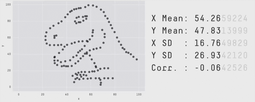
See also this supplementary page on plotting and degrees of freedom.

Announcements

Today

More on QRPs

Study 1 (Simmons et al., 2011)

we investigated whether listening to a children’s song induces an age contrast, making people feel older.

In exchange for payment, 30 University of Pennsylvania undergraduates sat at computer terminals, donned headphones, and were randomly assigned to listen to either a control song (“Kalimba,” an instrumental song by Mr. Scruff that comes free with the Windows 7 operating system) or a children’s song (“Hot Potato,” performed by The Wiggles).

After listening to part of the song, participants completed an ostensibly unrelated survey: They answered the question “How old do you feel right now?” by choosing among five options (very young, young, neither young nor old, old, and very old). They also reported their father’s age, allowing us to control for variation in baseline age across participants.

An analysis of covariance (ANCOVA) revealed the predicted effect: People felt older after listening to “Hot Potato” (adjusted M = 2.54 years) than after listening to the control song (adjusted M = 2.06 years), F(1, 27) = 5.06, p = .033.

Note

An analysis of covariance (ANCOVA) is a tool for asking whether there is some difference between groups (here the song listened to) when we account for a third variable, like their father’s age.

Link to supplemental illustration of ANCOVA

Study 2

we sought to conceptually replicate and extend Study 1. Having demonstrated that listening to a children’s song makes people feel older, Study 2 investigated whether listening to a song about older age makes people actually younger.

…we asked 20 University of Pennsylvania undergraduates to listen to either “When I’m Sixty-Four” by The Beatles or “Kalimba.” Then, in an ostensibly unrelated task, they indicated their birth date (mm/dd/yyyy) and their father’s age. We used father’s age to control for variation in baseline age across participants.

…An ANCOVA revealed the predicted effect: According to their birth dates, people were nearly a year-and-a-half younger after listening to “When I’m Sixty-Four” (adjusted M = 20.1 years) rather than to “Kalimba” (adjusted M = 21.5 years), F(1, 17) = 4.92, p = .040.

Wait a minute…

  • What did they say?
  • How is that even possible?

Illustration

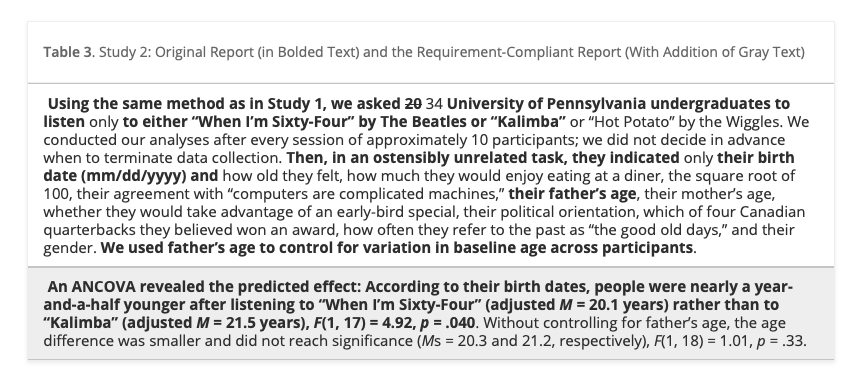
Table 3 from Simmons et al. (2011)

First, notice that in our original report, we redacted the many measures other than father’s age that we collected (including the dependent variable from Study 1: feelings of oldness). A reviewer would hence have been unable to assess the flexibility involved in selecting father’s age as a control. Second, by reporting only results that included the covariate, we made it impossible for readers to discover its critical role in achieving a significant result. Seeing the full list of variables now disclosed, reviewers would have an easy time asking for robustness checks, such as “Are the results from Study 1 replicated in Study 2?” They are not: People felt older rather than younger after listening to “When I’m Sixty-Four,” though not significantly so, F(1, 17) = 2.07, p = .168. Finally, notice that we did not determine the study’s termination rule in advance; instead, we monitored statistical significance approximately every 10 observations. Moreover, our sample size did not reach the 20-observation threshold set by our requirements.

The redacted version of the study we reported in this article fully adheres to currently acceptable reporting standards and is, not coincidentally, deceptively persuasive. The requirement-compliant version reported in Table 3 would be—appropriately—all but impossible to publish.

(Simmons et al., 2011)

Simulations

These simulations assessed the impact of four common degrees of freedom: flexibility in (a) choosing among dependent variables, (b) choosing sample size, (c) using covariates, and (d) reporting subsets of experimental conditions. We also investigated various combinations of these degrees of freedom.

We generated random samples with each observation independently drawn from a normal distribution, performed sets of analyses on each sample, and observed how often at least one of the resulting p values in each sample was below standard significance levels. For example, imagine a researcher who collects two dependent variables, say liking and willingness to pay. The researcher can test whether the manipulation affected liking, whether the manipulation affected willingness to pay, and whether the manipulation affected a combination of these two variables. The likelihood that one of these tests produces a significant result is at least somewhat higher than .05. We conducted 15,000 simulations of this scenario (and other scenarios) to estimate the size of “somewhat”.

(Simmons et al., 2011)

Findings

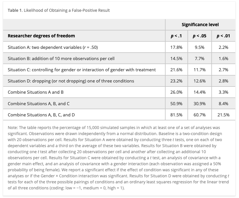
Table 1 from Simmons et al. (2011)

  • Researcher choices inflate false positive rates.

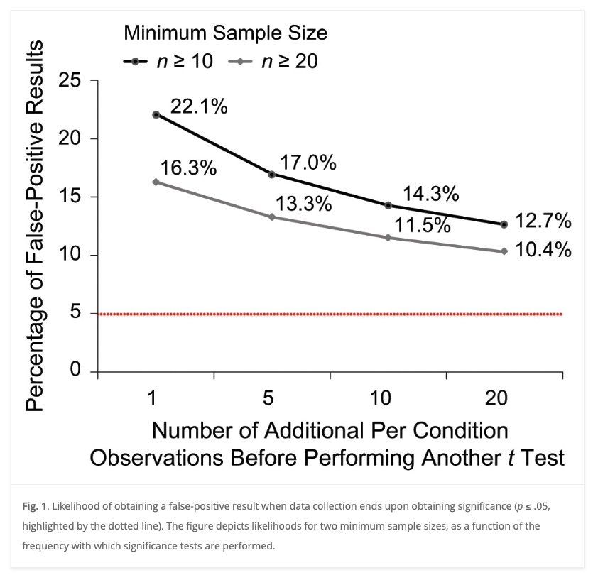
Figure 1 from Simmons et al. (2011)

  • Collecting more data after analyzing a small initial sample inflates the false positive rate.

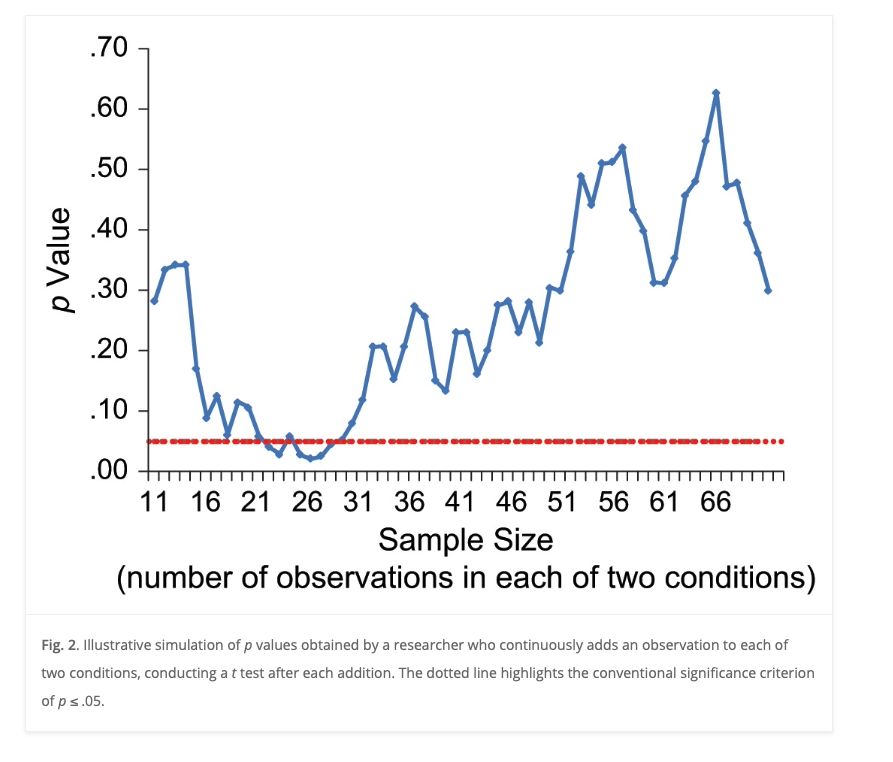
Figure 2 from Simmons et al. (2011)

  • Just because a statistical test met the criterion threshold with a small sample doesn’t mean it will do so with larger samples.

Recommendations

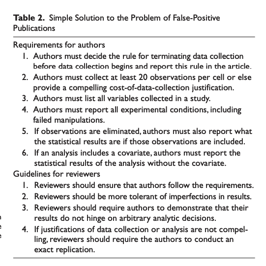
Table 2 from Simmons et al. (2011)

(Simmons et al., 2011)

Your thoughts?

  • Are these recommendations reasonable?
  • Are they feasible?
  • Do you think authors and reviewers will comply? Why or why not?

Reproducibility notes for (Simmons et al., 2011)

  • does not appear to have shared data or any supplementary materials along with the article.

Work session on p-hacking

p-hacking exercise

  • Enter (anonymized) data into a spreadsheet

https://docs.google.com/spreadsheets/d/1JI_Qih4wCzUrYTQYE3dpvVx2C7GdzfUZq0a3QhqQyeE/edit?usp=sharing

  • Choose a student_id (integer) for yourself (not your PSU ID or phone number)

Questions to discuss Monday

  • Who got a “significant” result?
  • How many different analyses did you try?
  • Who changed their analysis after finding a significant result?
  • Did anyone try another analysis–after you got a significant result–and keep the non-significant result?

Next time

Prevalence of QRPs - Read - (John, Loewenstein, & Prelec, 2012) - Class notes

Resources

References

John, L. K., Loewenstein, G., & Prelec, D. (2012). Measuring the prevalence of questionable research practices with incentives for truth telling. Psychological Science, 23(5), 524–532. https://doi.org/10.1177/0956797611430953
Matejka, J., & Fitzmaurice, G. (2017). Same stats, different graphs: Generating datasets with varied appearance and identical statistics through simulated annealing. In Proceedings of the 2017 CHI conference on human factors in computing systems (pp. 1290–1294). New York, NY, USA: Association for Computing Machinery. https://doi.org/10.1145/3025453.3025912
Simmons, J. P., Nelson, L. D., & Simonsohn, U. (2011). False-positive psychology: Undisclosed flexibility in data collection and analysis allows presenting anything as significant. Psychological Science, 22(11), 1359–1366. https://doi.org/10.1177/0956797611417632