---
title: "Discussion of Hadad et al. 2015"
format: html
---
## About
This document provides supporting information for the lab group discussion of @Hadad2015-qd.
## Setup
In order to generate images that support the concepts here, we set up a Python environment.
First, we install Python. We only run this once.
```{r}
#| eval: false
install.packages("reticulate")
library(reticulate)

# Installs a standalone Python version managed by reticulate (works cross-platform)
reticulate::install_python(version = "3.12")
reticulate::virtualenv_create(
  envname = "my_python_env",
  python = "3.12"
)
reticulate::virtualenv_install(
  envname = "my_python_env",
  packages = c("numpy", "matplotlib", "pandas", "scikit-learn")
)
```
Each time we render the file, we use the virtual environment we created in the previous step.
```{r}
reticulate::use_virtualenv("my_python_env", required = TRUE)
```
## Core question(s)
- Motion perception relates to clinical and development disorders.
- Motion perception/processing affects other aspect of perception.
- How does motion perception develop?
- When is it adult-like?
- What brain systems process motion?
## Key concepts
- Local vs. global motion
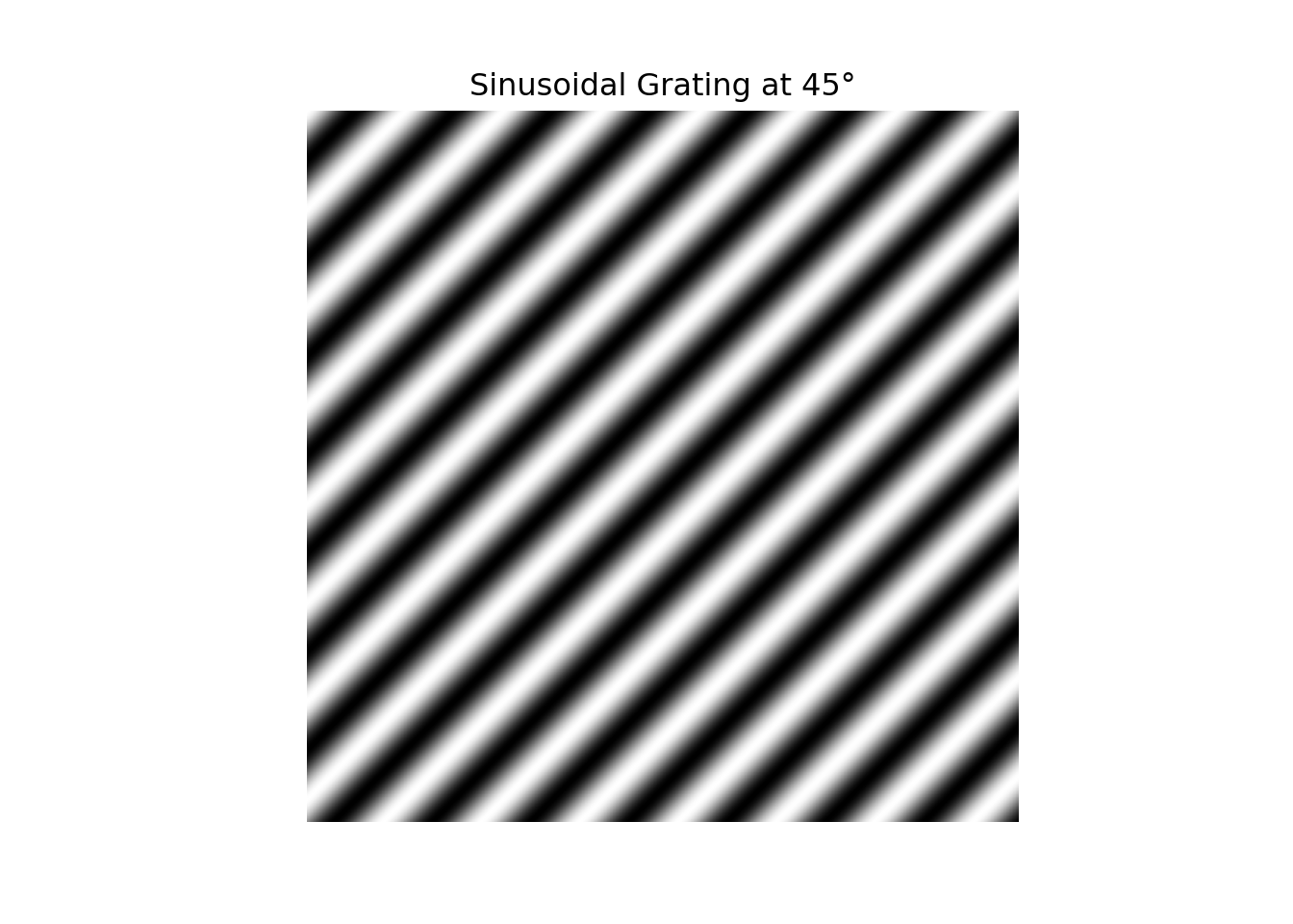
- Grating stimuli
```{python}
# Generated from Google AI query 2026-03-04
import numpy as np
import matplotlib.pyplot as plt
import math

def generate_sinusoidal_grating(size, spatial_frequency, angle=0, phase=0):
    """
    Generates a sinusoidal grating.

    Args:
        size (int): The width and height of the square grating in pixels.
        spatial_frequency (float): The spatial frequency (cycles per pixel,
                                   or inverse of wavelength in pixels).
        angle (float): The orientation of the grating in degrees.
        phase (float): The phase of the grating in degrees.

    Returns:
        numpy.ndarray: A 2D array representing the grating.
    """
    # Create a grid of coordinates
    x = np.arange(size)
    y = np.arange(size)
    X, Y = np.meshgrid(x, y)

    # Convert angle and phase to radians
    angle_rad = math.radians(angle)
    phase_rad = math.radians(phase)

    # Calculate the gradient along the specified angle
    # This creates a ramp that changes value along the desired orientation
    gradient = X * math.cos(angle_rad) + Y * math.sin(angle_rad)

    # Apply the sine wave function to the gradient
    # The result will range between -1 and 1
    grating = np.sin((2 * math.pi * gradient * spatial_frequency) + phase_rad)

    return grating

# --- Example Usage ---
# Parameters
grating_size = 512 # pixels
frequency = 0.02 # cycles per pixel (e.g. 1 cycle every 50 pixels)
orientation = 45 # degrees
start_phase = 90 # degrees

# Generate the grating
grating_pattern = generate_sinusoidal_grating(
    grating_size,
    frequency,
    orientation,
    start_phase
)

# Display the grating using Matplotlib
plt.imshow(grating_pattern, cmap='gray', vmin=-1, vmax=1)
plt.title(f"Sinusoidal Grating at {orientation}°")
plt.axis('off') # Hide axes
plt.show()
```

- A moving grating can yield a Barber Pole illusion:
![@Wikipedia-contributors2025-hv^["By The original uploader was Rokers at English Wikipedia. - Transferred from en.wikipedia to Commons., CC BY-SA 3.0, https://commons.wikimedia.org/w/index.php?curid=1881350"]](https://upload.wikimedia.org/wikipedia/commons/3/39/Barberpole_illusion_animated.gif){#fig-barber-pole-gif}
- Plaids
::: {#fig-plaids-ambiguous-not}
<iframe width="560" height="315" src="https://www.youtube.com/embed/WhbZesV2GRk?si=TeA4BPTaGS7Dz6bs" title="YouTube video player" frameborder="0" allow="accelerometer; autoplay; clipboard-write; encrypted-media; gyroscope; picture-in-picture; web-share" referrerpolicy="strict-origin-when-cross-origin" allowfullscreen></iframe>
@ricardomartins2016-pt
:::
- Dot stimuli
- Random Dot Kinematograms (RDKs)
- [Example](https://databrary.org/volume/49) from Databrary
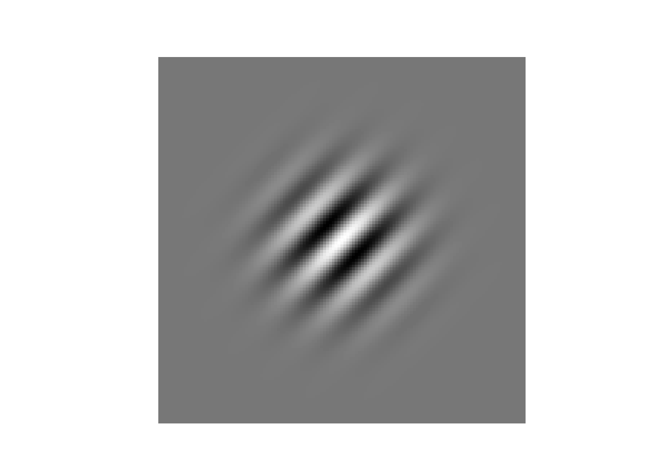
- Gabor stimuli (Gabor patch)
- A grating convolved with^[@Wikipedia-contributors2026-aa] a 2D Gaussian^[@Wikipedia-contributors2026-rw].
```{python}
# Generated from Safari AI query 2026-03-18
import numpy as np
import matplotlib.pyplot as plt

def make_gabor_patch(size, sigma, wavelength, orientation, phase, gamma):
    """
    Generates a Gabor patch.

    Parameters:
    size (int): The size of the patch in pixels (e.g., 128).
    sigma (float): The spatial constant (standard deviation of the Gaussian envelope).
    wavelength (float): The wavelength of the sine wave (spatial frequency).
    orientation (float): The orientation of the patch in degrees.
    phase (float): The phase of the sine wave in degrees.
    gamma (float): The spatial aspect ratio (1 for circular, <1 for elliptical).
    """
    # Convert parameters to radians
    theta = np.deg2rad(orientation)
    psi = np.deg2rad(phase)

    # Calculate sigma_x and sigma_y based on aspect ratio
    sigma_x = sigma
    sigma_y = sigma / gamma

    # Create a meshgrid of coordinates
    # The range is chosen to ensure the Gaussian envelope is fully captured (typically +/- 3*sigma)
    nstds = 3
    xmax = max(abs(nstds * sigma_x * np.cos(theta)), abs(nstds * sigma_y * np.sin(theta)))
    ymax = max(abs(nstds * sigma_x * np.sin(theta)), abs(nstds * sigma_y * np.cos(theta)))
    xmax = int(np.ceil(max(1, xmax)))
    ymax = int(np.ceil(max(1, ymax)))
    xmin, ymin = -xmax, -ymax

    # Expand the range if the specified size is larger
    if size > 2 * xmax + 1:
        xmax = ymax = (size - 1) // 2
        xmin, ymin = -xmax, -ymax

    [x, y] = np.meshgrid(np.arange(xmin, xmax + 1), np.arange(ymin, ymax + 1))

    # Rotate the coordinates
    x_theta = x * np.cos(theta) + y * np.sin(theta)
    y_theta = -x * np.sin(theta) + y * np.cos(theta)

    # Generate the Gabor patch
    # Gaussian envelope
    gauss = np.exp(-0.5 * (x_theta**2 / sigma_x**2 + y_theta**2 / sigma_y**2))
    # Sine wave grating
    sine = np.cos(2 * np.pi / wavelength * x_theta + psi)
    # Combine to form the Gabor patch
    gabor_patch = gauss * sine

    return gabor_patch

# --- Example Usage ---
gabor_data = make_gabor_patch(
    size=128,          # Image size in pixels
    sigma=15.0,        # Gaussian standard deviation
    wavelength=15.0,   # Wavelength of sine wave
    orientation=45,    # Orientation in degrees (45 for diagonal)
    phase=0,           # Phase in degrees (0 for cosine phase)
    gamma=1.0          # Aspect ratio (1 for circular)
)

# Display the Gabor patch using matplotlib with no interpolation to show raw pixels
plt.imshow(gabor_data, cmap='gray', interpolation='none')
plt.axis('off') # Hide axes
plt.show()
```
```{python}
import numpy as np
import matplotlib.pyplot as plt
import matplotlib.animation as animation

# Function to create Gabor patch
def create_gabor(size, sigma, theta, lam, psi, gamma):
    # Standard Gabor filter formula [14]
    y, x = np.meshgrid(np.linspace(-1,1,size), np.linspace(-1,1,size))
    x_theta = x * np.cos(theta) + y * np.sin(theta)
    y_theta = -x * np.sin(theta) + y * np.cos(theta)

    gb = np.exp(-.5 * (x_theta**2 + gamma**2 * y_theta**2) / sigma**2) \
         * np.cos(2 * np.pi * x_theta / lam + psi)
    return gb

# Animation
fig, ax = plt.subplots()
gabor = create_gabor(100, 0.4, 0, 10, 0, 1)
im = ax.imshow(gabor, cmap='gray', animated=True, vmin=-1, vmax=1)

def update(i):
    # Update phase to move
    new_gabor = create_gabor(100, 0.4, 0, 10, i/10.0, 1)
    im.set_array(new_gabor)
    return im,

ani = animation.FuncAnimation(fig, update, interval=20)
plt.show()
```