flowchart TD
  A[Collect] --> B[Gather]
  B --> C[Clean]
  C --> B
  C --> D[Visualize]
  D --> C
  D --> E[Analyze]
  E --> C
Making plots with ggplot2
2025-03-27
Rick Gilmore
Prelude
In the news…

https://reddit.com/r/spaceporn

https://reddit.com/r/dataisbeautiful

https://reddit.com/r/dataisbeautiful
Announcements
- Exercise 06 available
- On AI and academic work
Feynman (1974)
“The first principle is that you must not fool yourself—and you are the easiest person to fool. So you have to be very careful about that…”

Today’s topics
- Data processing workflows
- Intro to
ggplot2 - Introducing posit.cloud
- Work session
Data workflow
- Collect
- Gather
- Clean
- Visualize
- Analyze
Data workflow (more realistic)
Targets
- A data frame
- Rectangular
- Tidy (rows are observations, columns are variables); Hadley Wickham (2014)
- Short, evocative variable names
How script?
- Save commands in a file (
*.R) - Save commands and comments in a Quarto file (
*.qmd)- See the ‘Learning-Quarto’ assignment on posit.cloud
About ggplot2
Set-up
- Load package(s)
Acquire data
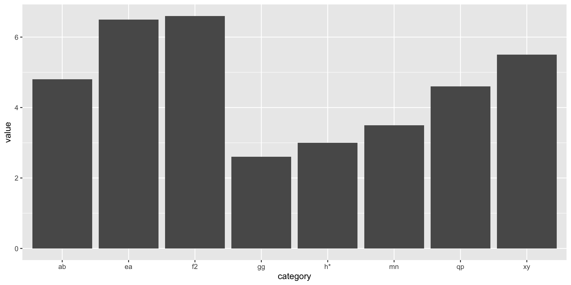
  category value
1       ab   4.8
2       xy   5.5
3       mn   3.5
4       qp   4.6
5       ea   6.5
6       f2   6.6
7       gg   2.6
8       h*   3.0
Examine data
'data.frame':   8 obs. of  2 variables:
 $ category: chr  "ab" "xy" "mn" "qp" ...
 $ value   : num  4.8 5.5 3.5 4.6 6.5 6.6 2.6 3
Step by step

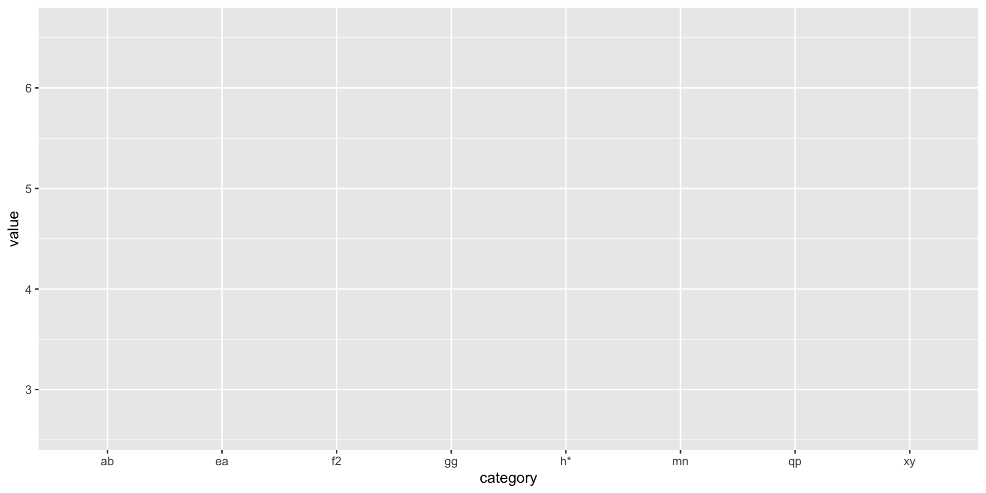
Adding aesthetics
Adding a ‘geom’
Adding a fill color
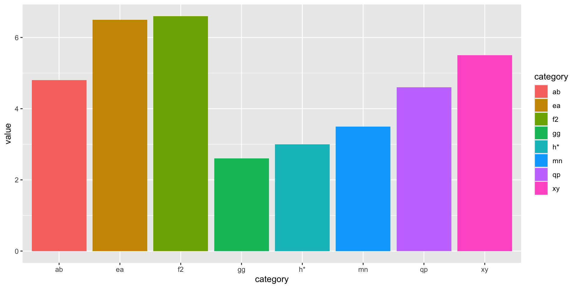
Figure 4: Adding an aesthetic based on ‘category’ to fill the bars with color.
All at once

Figure 5: The same figure generated from a short sequence of commands.
Why sequential?
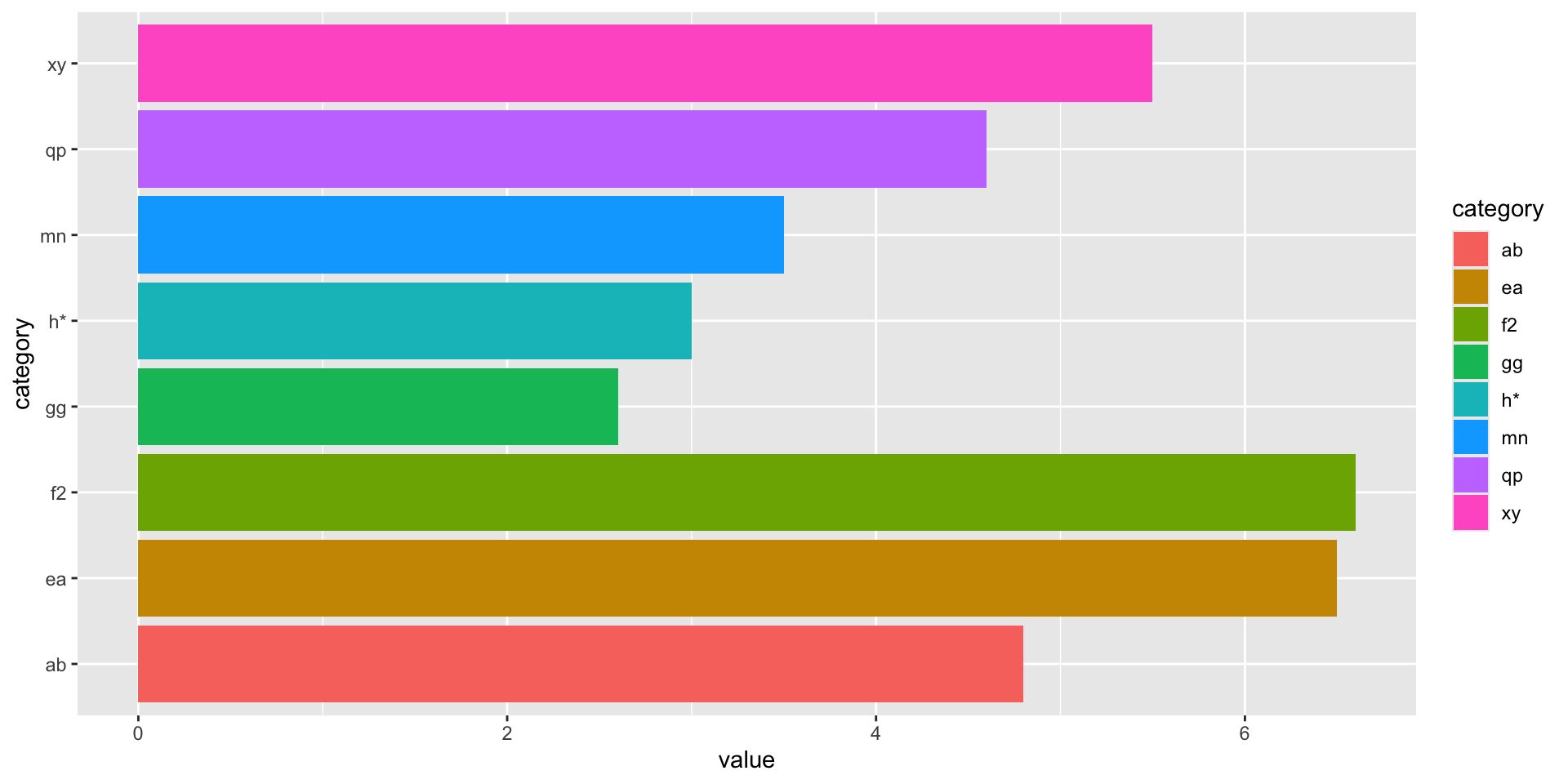
Figure 6: Colored column with flipped axes
versus…

Figure 7: Colored column with flipped axes
Change geom
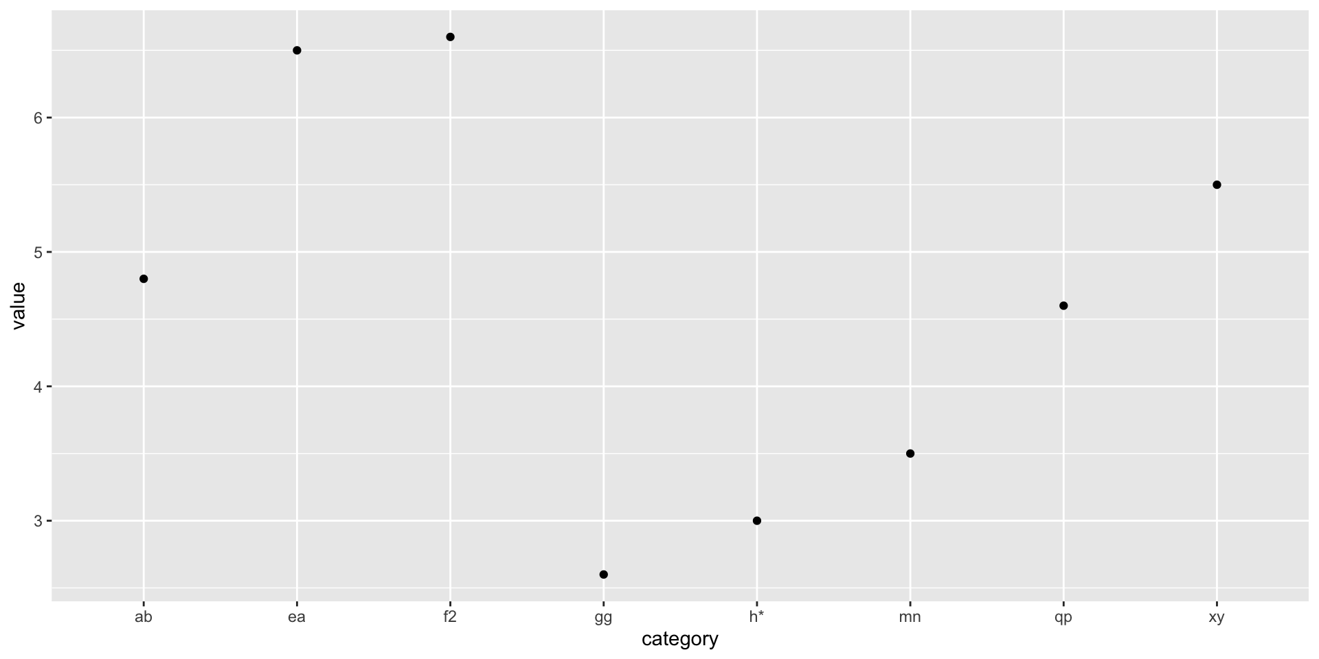
Figure 8: Colored column with flipped axes
Style recommendation
A personal story
Qian, Berenbaum, & Gilmore (2022)
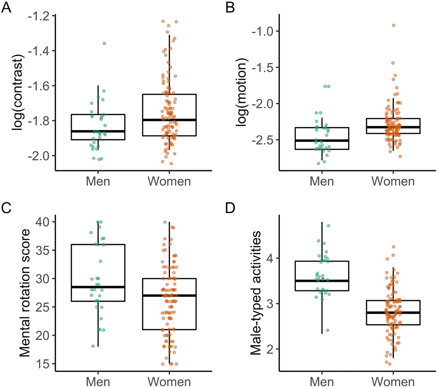
Figure 1 from Qian et al. (2022)
Script everything…
- You possibly can
- Re-use and recycle
- https://github.com/gilmore-lab/sex-differences-project
“Stand on the shoulders of giants”
- Wikipedia contributors (2024)

giphy.com
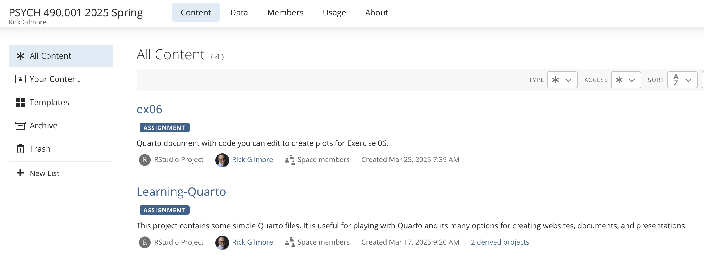
Introducing posit.cloud
Resources
References
Feynman, R. P. (1974). Cargo cult science. Retrieved from https://calteches.library.caltech.edu/51/2/CargoCult.htm
Hadley Wickham. (2014). Tidy data | wickham | journal of statistical software. https://doi.org/10.18637/jss.v059.i10
Qian, Y., Berenbaum, S. A., & Gilmore, R. O. (2022). Vision contributes to sex differences in spatial cognition and activity interests. Scientific Reports, 12, 17623. https://doi.org/10.1038/s41598-022-22269-y
Wickham, H., Navarro, D., & Pedersen, T. L. (n.d.). ggplot2: Elegant graphics for data analysis (3e). Retrieved January 12, 2025, from https://ggplot2-book.org/
Wikipedia contributors. (2024, December 10). Standing on the shoulders of giants. Retrieved from https://en.wikipedia.org/wiki/Standing_on_the_shoulders_of_giants
Wilkinson, L., Wills, D., Rope, D., Norton, A., & Dubbs, R. (2005). The grammar of graphics (statistics and computing) (2nd edition). Springer. Retrieved from https://www.amazon.com/Grammar-Graphics-Statistics-Computing/dp/0387245448
