Introduction to Python

2025-04-03

Rick Gilmore

Prelude

EllaFitzgeraldVEVO (2024)

Overview

In the news

Figure from Witze (2025)

Kozlov (2025)

Mandavilli & Rabin (2025)

Nunn (2025)

“Leading Causes of Death” (2024)

Causes of Death, 2018-2023, 20-24 year-olds

Cause	Deaths	Crude Rate
Accidents (unintentional injuries)	56981	43.4
Intentional self-harm (suicide)	23238	17.7
Assault (homicide)	20098	15.3

Source: CDC Wonder

Cause	Deaths	Crude Rate
Malignant neoplasms	4627	3.5
Diseases of heart	3520	2.7
COVID-19	1779	1.4
Diabetes mellitus	1259	1.0

Source: CDC Wonder

Cause	Deaths	Crude Rate
Congenital malformations, deformations and chromosomal abnormalities	1217	0.9
Pregnancy, childbirth and the puerperium	826	0.6
Chronic lower respiratory diseases	699	0.5
Influenza and pneumonia	634	0.5

Source: CDC Wonder

Cause	Deaths	Crude Rate
Cerebrovascular diseases	619	0.5
Legal intervention	451	0.3
Septicemia	432	0.3
Nephritis, nephrotic syndrome and nephrosis	289	0.2

Source: CDC Wonder

Announcements

Exercise 06 due today.
Final project presentation survey due Tuesday, April 8.

Tentative presentation schedule

supplemental/presentation-schedule

Last time…

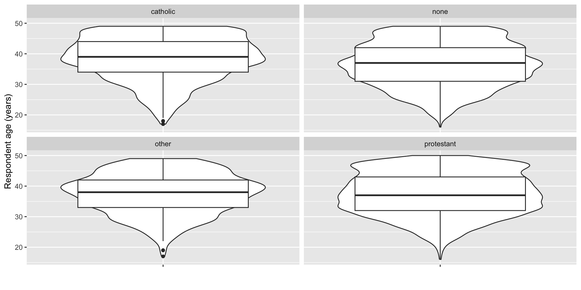
NSFG repondent age by religion figure

Recommended design principles

Work iteratively (in small steps)
Keep prior versions
- Store figure code in *.R or *.qmd files
No ‘secret sauce’
The process is the product

Today

Introduction to Python
Work session
- DataCamp
- Exercise 06
- Final projects

Introduction to Python

Why learn Python?

It’s fun
It’s free
Amaze your friends; dazzle your rivals
Powerful tool
It will make you a more productive researcher
Practical job-related skill
More popular than R!

Why should psychologists learn Python?

Make experiments using Psychopy
Gather, clean, visualize your data using matplotlib, Seaborn, etc.
Reproducible == robust, easy to share with others

Console

R

license()


This software is distributed under the terms of the GNU General
Public License, either Version 2, June 1991 or Version 3, June 2007.
The terms of version 2 of the license are in a file called COPYING
which you should have received with
this software and which can be displayed by RShowDoc("COPYING").
Version 3 of the license can be displayed by RShowDoc("GPL-3").

Copies of both versions 2 and 3 of the license can be found
at https://www.R-project.org/Licenses/.

A small number of files (the API header files listed in
R_DOC_DIR/COPYRIGHTS) are distributed under the
LESSER GNU GENERAL PUBLIC LICENSE, version 2.1 or later.
This can be displayed by RShowDoc("LGPL-2.1"),
or obtained at the URI given.
Version 3 of the license can be displayed by RShowDoc("LGPL-3").

'Share and Enjoy.'

Python

license

See https://www.python.org/psf/license/

Reminder

Painful lesson #1

Computers are super-literal. They are anally literal. More anally literal than any human being you’ve ever had to deal with.

You’re not going to change them. Being this anal is their superpower.

Just deal.

Simple math

R

x <- c(1, 4, 7)
sum(x)

[1] 12

Python

x = [1, 4, 7]
sum(x)

Getting help

R

help("sort")

Python

help("numpy.sort")

Help on _ArrayFunctionDispatcher in numpy:

numpy.sort = sort(a, axis=-1, kind=None, order=None, *, stable=None)
    Return a sorted copy of an array.

    Parameters
    ----------
    a : array_like
        Array to be sorted.
    axis : int or None, optional
        Axis along which to sort. If None, the array is flattened before
        sorting. The default is -1, which sorts along the last axis.
    kind : {'quicksort', 'mergesort', 'heapsort', 'stable'}, optional
        Sorting algorithm. The default is 'quicksort'. Note that both 'stable'
        and 'mergesort' use timsort or radix sort under the covers and,
        in general, the actual implementation will vary with data type.
        The 'mergesort' option is retained for backwards compatibility.
    order : str or list of str, optional
        When `a` is an array with fields defined, this argument specifies
        which fields to compare first, second, etc.  A single field can
        be specified as a string, and not all fields need be specified,
        but unspecified fields will still be used, in the order in which
        they come up in the dtype, to break ties.
    stable : bool, optional
        Sort stability. If ``True``, the returned array will maintain
        the relative order of ``a`` values which compare as equal.
        If ``False`` or ``None``, this is not guaranteed. Internally,
        this option selects ``kind='stable'``. Default: ``None``.

        .. versionadded:: 2.0.0

    Returns
    -------
    sorted_array : ndarray
        Array of the same type and shape as `a`.

    See Also
    --------
    ndarray.sort : Method to sort an array in-place.
    argsort : Indirect sort.
    lexsort : Indirect stable sort on multiple keys.
    searchsorted : Find elements in a sorted array.
    partition : Partial sort.

    Notes
    -----
    The various sorting algorithms are characterized by their average speed,
    worst case performance, work space size, and whether they are stable. A
    stable sort keeps items with the same key in the same relative
    order. The four algorithms implemented in NumPy have the following
    properties:

    =========== ======= ============= ============ ========
       kind      speed   worst case    work space   stable
    =========== ======= ============= ============ ========
    'quicksort'    1     O(n^2)            0          no
    'heapsort'     3     O(n*log(n))       0          no
    'mergesort'    2     O(n*log(n))      ~n/2        yes
    'timsort'      2     O(n*log(n))      ~n/2        yes
    =========== ======= ============= ============ ========

    .. note:: The datatype determines which of 'mergesort' or 'timsort'
       is actually used, even if 'mergesort' is specified. User selection
       at a finer scale is not currently available.

    For performance, ``sort`` makes a temporary copy if needed to make the data
    `contiguous <https://numpy.org/doc/stable/glossary.html#term-contiguous>`_
    in memory along the sort axis. For even better performance and reduced
    memory consumption, ensure that the array is already contiguous along the
    sort axis.

    The sort order for complex numbers is lexicographic. If both the real
    and imaginary parts are non-nan then the order is determined by the
    real parts except when they are equal, in which case the order is
    determined by the imaginary parts.

    Previous to numpy 1.4.0 sorting real and complex arrays containing nan
    values led to undefined behaviour. In numpy versions >= 1.4.0 nan
    values are sorted to the end. The extended sort order is:

      * Real: [R, nan]
      * Complex: [R + Rj, R + nanj, nan + Rj, nan + nanj]

    where R is a non-nan real value. Complex values with the same nan
    placements are sorted according to the non-nan part if it exists.
    Non-nan values are sorted as before.

    quicksort has been changed to:
    `introsort <https://en.wikipedia.org/wiki/Introsort>`_.
    When sorting does not make enough progress it switches to
    `heapsort <https://en.wikipedia.org/wiki/Heapsort>`_.
    This implementation makes quicksort O(n*log(n)) in the worst case.

    'stable' automatically chooses the best stable sorting algorithm
    for the data type being sorted.
    It, along with 'mergesort' is currently mapped to
    `timsort <https://en.wikipedia.org/wiki/Timsort>`_
    or `radix sort <https://en.wikipedia.org/wiki/Radix_sort>`_
    depending on the data type.
    API forward compatibility currently limits the
    ability to select the implementation and it is hardwired for the different
    data types.

    Timsort is added for better performance on already or nearly
    sorted data. On random data timsort is almost identical to
    mergesort. It is now used for stable sort while quicksort is still the
    default sort if none is chosen. For timsort details, refer to
    `CPython listsort.txt
    <https://github.com/python/cpython/blob/3.7/Objects/listsort.txt>`_
    'mergesort' and 'stable' are mapped to radix sort for integer data types.
    Radix sort is an O(n) sort instead of O(n log n).

    NaT now sorts to the end of arrays for consistency with NaN.

    Examples
    --------
    >>> import numpy as np
    >>> a = np.array([[1,4],[3,1]])
    >>> np.sort(a)                # sort along the last axis
    array([[1, 4],
           [1, 3]])
    >>> np.sort(a, axis=None)     # sort the flattened array
    array([1, 1, 3, 4])
    >>> np.sort(a, axis=0)        # sort along the first axis
    array([[1, 1],
           [3, 4]])

    Use the `order` keyword to specify a field to use when sorting a
    structured array:

    >>> dtype = [('name', 'S10'), ('height', float), ('age', int)]
    >>> values = [('Arthur', 1.8, 41), ('Lancelot', 1.9, 38),
    ...           ('Galahad', 1.7, 38)]
    >>> a = np.array(values, dtype=dtype)       # create a structured array
    >>> np.sort(a, order='height')                        # doctest: +SKIP
    array([('Galahad', 1.7, 38), ('Arthur', 1.8, 41),
           ('Lancelot', 1.8999999999999999, 38)],
          dtype=[('name', '|S10'), ('height', '<f8'), ('age', '<i4')])

    Sort by age, then height if ages are equal:

    >>> np.sort(a, order=['age', 'height'])               # doctest: +SKIP
    array([('Galahad', 1.7, 38), ('Lancelot', 1.8999999999999999, 38),
           ('Arthur', 1.8, 41)],
          dtype=[('name', '|S10'), ('height', '<f8'), ('age', '<i4')])

Importing packages/libraries

R

1if (!require(ggplot2)) {
2  install.packages("ggplot2")
} else {
  message("Already installed.")
}
3library(ggplot2)

1: If the package isn’t installed…
2: Install it (from the internet).
3: Load the package into memory

Python

1<Install library outside of Python>
2import numpy as np

1: Not shown here, sorry.
2: Load the numpy library into memory. We (optionally) give it a short name.

`sort()` again

R

x <- c(7, 1, 4, 12)
sort(x)

[1]  1  4  7 12

Python

1x = np.array([7, 1, 4, 12])
2np.sort(x)

1: Create a numpy array.
2: Call the numpy sort function/method on x.

array([ 1,  4,  7, 12])

R

your_age <- 21
your_shoe_size <- 8.5

your_age + your_shoe_size

your_shoe_size/your_age

[1] 29.5

[1] 0.4047619

Python

your_age = 21
your_shoe_size = 8.5

your_age + your_shoe_size

your_shoe_size/your_age

[1] 29.5

[1] 0.4047619

R

Don’t use =, use <-

You can substitute = but don’t. Use <-.
It’s stylistic, but style matters.
It’s like saying ‘like’ all the time. Like people will like understand you, but they’ll wonder why you like say like all the time when you really need not.
It’s also a topic that could get you in a ‘flame war’.
Avoid flame wars if you can. Life is too short.

Python

Use =, not <-

It’s essential.

Asking questions

comparison operators (==, !=, >, <, etc.).

R

1 == 0
sqrt(9) < 4

[1] FALSE

[1] TRUE

Python

1 == 0
1np.sqrt(9) < 4

1: Have to use numpy to get the square root (sqrt) function.

False

np.True_

What can we talk about?

Strings

R

c('w', 'x', 'y', 'z')

middle_letters <- c('m', 'n', 'o')
middle_letters

[1] "w" "x" "y" "z"

[1] "m" "n" "o"

Python

['w', 'x', 'y', 'z']

middle_letters = ['m', 'n', 'o']
middle_letters

['w', 'x', 'y', 'z']

['m', 'n', 'o']

Strings \(\neq\) numbers!

R

1identical(c('1', '2'), c(1, 2))

1: Safe way in R to compare things.

[1] FALSE

Python

['1', '2'] == [1, 2]

False

Note

R uses FALSE where Python uses False.

Data frames

R

df <- data.frame(name = c("Tom", "Jerry"), 
  age = c(10, 19))
str(df)

'data.frame':   2 obs. of  2 variables:
 $ name: chr  "Tom" "Jerry"
 $ age : num  10 19

Python

1import pandas as pd
data = {'name': ["Tom", "Jerry"], 
  'age': [10, 19]}
df = pd.DataFrame(data)
print(df)

1: Load the pandas package to handle data frames.

    name  age
0    Tom   10
1  Jerry   19

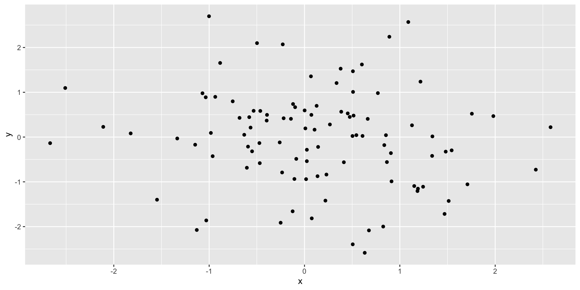
Plots in R

rand_x <- rnorm(100)
rand_y <- rnorm(100)
df <- data.frame(x = rand_x, y = rand_y)
df |>
  ggplot() +
  aes(x = x, y = y) +
  geom_point()

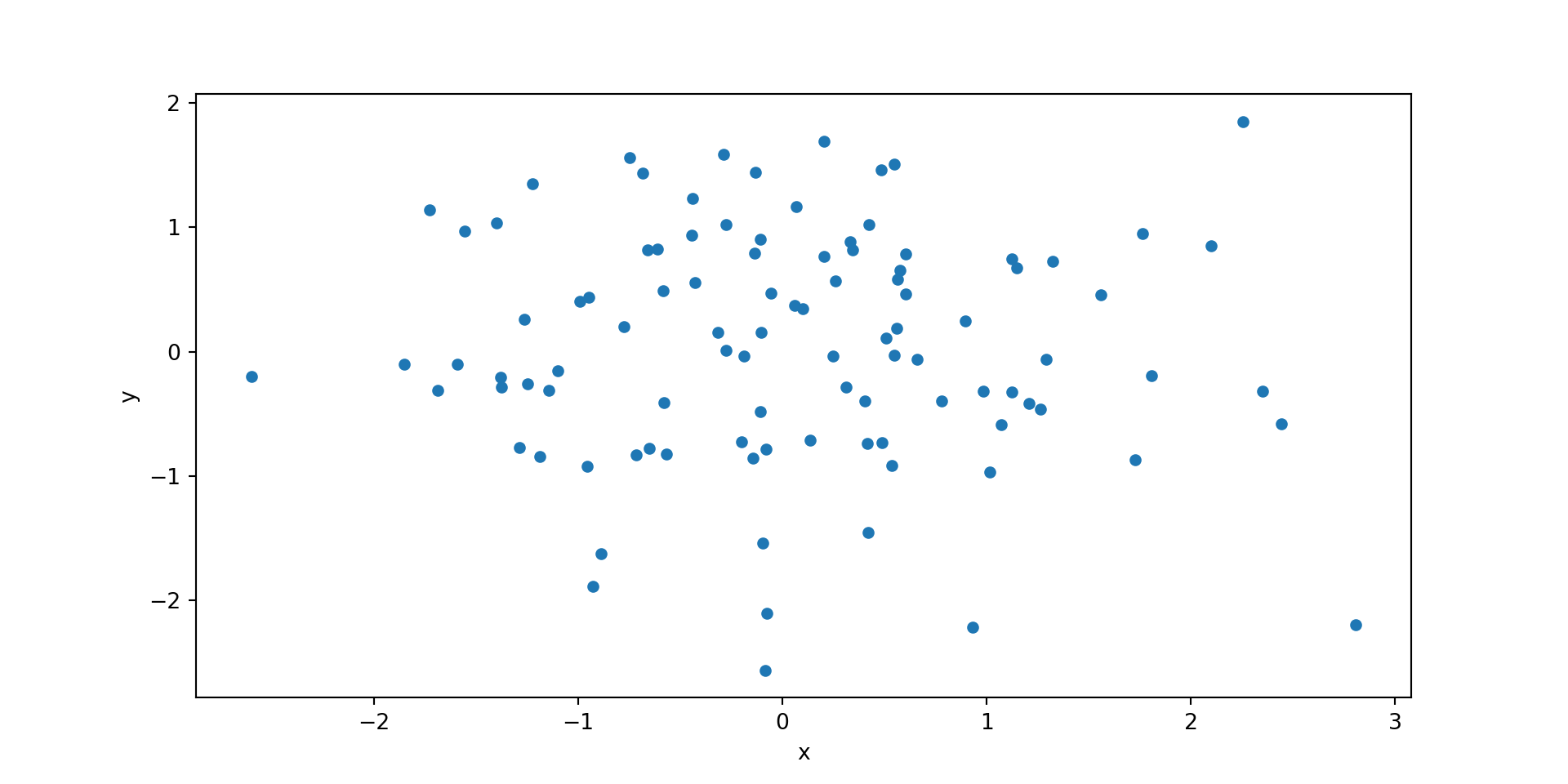
Plots in Python

1import matplotlib.pyplot as plt
rand_x = np.random.normal(0, 1, 100)
rand_y = np.random.normal(0, 1, 100)
data = {'x': rand_x, 'y': rand_y}
df = pd.DataFrame(data)
df.plot(x = 'x', y = 'y', kind = 'scatter')
plt.show()

1: Import pyplot module from matplotlib with short name plt.

Tip to the wise

R

# Load packages into memory
library(ggplot2)
library(dplyr)
library(readr)

Python

# Import libraries and modules
import numpy as np
import matplotlib.pyplot as plt
import pandas as pd

Load/import packages/libraries once
At the top of your script/document
Need a new one? Add it to the code at the top of your script/document.

Rules for naming things

Replace spaces (and hyphens/minus characters -) with underscores (_), and
Start names with letters, not numbers.

acceptable names for things: bigly, good_name, a_longer_good_name, Good_name1, and even thisIsCamelCaseNoUnderscores
unacceptable names: !good, bad name (has a space) or 1_very_bad_name (starts with a number).

Work session

Next time

Exploring data with Python

Resources

References

EllaFitzgeraldVEVO. (2024). Ella fitzgerald, louis armstrong - let’s call the whole thing off (audio). Youtube. Retrieved from https://www.youtube.com/watch?v=qfu_PD-7EtM

Kozlov, M. (2025). ’One of the darkest days’: NIH purges agency leadership amid mass layoffs. Nature. https://doi.org/10.1038/d41586-025-01016-z

Leading Causes of Death. (2024, October 26). Retrieved April 3, 2025, from https://www.cdc.gov/nchs/fastats/leading-causes-of-death.htm

Mandavilli, A., & Rabin, R. C. (2025, April 2). C.D.C. Cuts threaten to set back the nation’s health, critics say. The New York Times. The New York Times. Retrieved from https://www.nytimes.com/2025/04/02/health/cdc-layoffs-kennedy.html

Nunn, E. B. (2025, April 2). Inside the C.D.C., a final “love letter” before mass layoffs. The New York Times. The New York Times. Retrieved from https://www.nytimes.com/2025/04/02/health/cdc-layoffs-response.html

Witze, A. (2025). 75% of US scientists who answered nature poll consider leaving. Nature. https://doi.org/10.1038/d41586-025-00938-y

Introduction to Python

Prelude

Overview

In the news

Causes of Death, 2018-2023, 20-24 year-olds

Announcements

Tentative presentation schedule

Last time…

Recommended design principles

Today

Introduction to Python

Why learn Python?

Why should psychologists learn Python?

Console

R

Python

Reminder

Simple math

R

Python

Getting help

R

Python

Importing packages/libraries

R

Python

sort() again

R

Python

R

Python

R

Python

Asking questions

R

Python

What can we talk about?

Strings

R

Python

Strings \(\neq\) numbers!

R

Python

Data frames

R

Python

Plots in R

Plots in Python

Tip to the wise

R

Python

Rules for naming things

Work session

Next time

Resources

References

`sort()` again