On p-hacking

Purpose

This document summarizes an analyis of the p-hacking exercise. In it, we gather data about what individual students did and try to make sense of it.

Quantitative analysis

It often saves typing to load a set of commands into memory. In R, groups of useful commands are called ‘packages’. We can load a set of useful packages into memory by issuing the following command:

library(tidyverse)

── Attaching core tidyverse packages ──────────────────────── tidyverse 2.0.0 ──
✔ dplyr     1.1.3     ✔ readr     2.1.4
✔ forcats   1.0.0     ✔ stringr   1.5.1
✔ ggplot2   3.4.4     ✔ tibble    3.2.1
✔ lubridate 1.9.3     ✔ tidyr     1.3.0
✔ purrr     1.0.2     
── Conflicts ────────────────────────────────────────── tidyverse_conflicts() ──
✖ dplyr::filter() masks stats::filter()
✖ dplyr::lag()    masks stats::lag()
ℹ Use the conflicted package (<http://conflicted.r-lib.org/>) to force all conflicts to become errors

Note

If you are interested in a career related to data science, tidyverse is a very powerful set of tools you will want to know more about.

Data entry

Via a Google Sheet: https://docs.google.com/spreadsheets/d/1fnSwFrUcKvgqq_agDLe4t2DHXHtHoOlmLdtLVRSemrI/edit?usp=sharing

Note

Gilmore added data validation (Format/Data Validation) to the columns. Why?

---

Note

These data are “long”. Each row is a unique observation. Long data are often easier to work with. But not always.

Data gathering

First, I authenticate (sign-in) to Google using my Gmail account. If I haven’t logged in using this script recently, it will ask me to log-in again.

googledrive::drive_auth("rick.o.gilmore@gmail.com")

Then I download the Google Sheet to a directory/folder called csv/ using the file name p-hacking-fa23.csv.

googledrive::drive_download(file = "PSYCH 490.009 2023 Fall P-hacking", path = "csv/p-hacking-fa23.csv", type = 'csv', overwrite = TRUE)

File downloaded:

• 'PSYCH 490.009 2023 Fall P-hacking'
  <id: 1JI_Qih4wCzUrYTQYE3dpvVx2C7GdzfUZq0a3QhqQyeE>

Saved locally as:

• 'csv/p-hacking-fa23.csv'

Note

What does CSV mean?

Why are CSV files often used in data analysis?

One answer is that CSV files are inter-operable and largely reusable, two of the characteristics recommended for sharing data under the FAIR principles (Wilkinson et al., 2016).

Next, I read the CSV file using the read_csv() function.

p_hacking_fa23 <- read_csv(file = "csv/p-hacking-fa23.csv", show_col_types = FALSE)

Note

Functions in R take inputs and deliver outputs. The inputs are file and show_col_types.

The output is an object called p_hacking. It is a table of data that I can refer to with that name.

I like to use the ‘structure’ function or str() to see what the data look like.

Note

Data is a plural noun. So, (when we don’t forget this) we say ‘The data are…’ not ‘The data is…’.

str(p_hacking_fa23)

spc_tbl_ [16 × 16] (S3: spec_tbl_df/tbl_df/tbl/data.frame)
 $ student           : num [1:16] 0 12 37 37 37 12 66 66 66 94 ...
 $ analysis          : num [1:16] 1 1 1 2 3 2 1 2 3 1 ...
 $ party             : chr [1:16] "democrats" "republicans" "republicans" "democrats" ...
 $ prediction        : chr [1:16] "worse" "better" "better" "better" ...
 $ power_president   : logi [1:16] FALSE TRUE FALSE FALSE TRUE TRUE ...
 $ power_governors   : logi [1:16] FALSE FALSE FALSE FALSE FALSE FALSE ...
 $ power_senators    : logi [1:16] TRUE TRUE TRUE FALSE FALSE TRUE ...
 $ power_reps        : logi [1:16] TRUE TRUE TRUE TRUE FALSE TRUE ...
 $ econ_employment   : logi [1:16] TRUE FALSE TRUE TRUE TRUE FALSE ...
 $ econ_inflation    : logi [1:16] FALSE TRUE FALSE TRUE TRUE TRUE ...
 $ econ_gdp          : logi [1:16] FALSE FALSE FALSE TRUE FALSE TRUE ...
 $ econ_stocks       : logi [1:16] TRUE TRUE TRUE FALSE FALSE TRUE ...
 $ factor_in_power   : logi [1:16] FALSE FALSE FALSE TRUE FALSE FALSE ...
 $ exclude_recessions: logi [1:16] FALSE TRUE FALSE TRUE FALSE TRUE ...
 $ p_value           : num [1:16] 0.06 0.01 0.01 0.07 0.01 0.27 0.01 0.36 0.01 0.03 ...
 $ publishable       : chr [1:16] "no" "yes" "yes" "no" ...
 - attr(*, "spec")=
  .. cols(
  ..   student = col_double(),
  ..   analysis = col_double(),
  ..   party = col_character(),
  ..   prediction = col_character(),
  ..   power_president = col_logical(),
  ..   power_governors = col_logical(),
  ..   power_senators = col_logical(),
  ..   power_reps = col_logical(),
  ..   econ_employment = col_logical(),
  ..   econ_inflation = col_logical(),
  ..   econ_gdp = col_logical(),
  ..   econ_stocks = col_logical(),
  ..   factor_in_power = col_logical(),
  ..   exclude_recessions = col_logical(),
  ..   p_value = col_double(),
  ..   publishable = col_character()
  .. )
 - attr(*, "problems")=<externalptr> 

Questions to explore

• Most data analysts find that the process of exploring data is iterative.
• We start with a question. That leads to another question. That leads to yet another question.
• It is also sometimes cyclical. To answer a question requires that we modify the form of our data file.
• I like to start with thinking about “data pictures.” If X was true, what would the data look like?

Note

So, what are our questions?

What view of the data would help us answer them?

Visualize

Party by prediction

xtabs(formula = ~ party + prediction, data = p_hacking_fa23)

             prediction
party         better worse
  democrats        6     1
  republicans      5     4

p_hacking_fa23 |>
  ggplot() +
  aes(x = party, fill = prediction) +
  geom_bar() +
  theme_classic() +
  ylab("n respondents")

Figure 1: Party chosen by prediction: PSYCH 490 Fall 2023

p_hacking_fa23 |>
  ggplot() +
  aes(x = p_value, fill = party) +
  geom_histogram(bins = 10) +
  facet_grid(~ prediction)

Figure 2: Histogram of realized p values by party chosen: PSYCH 490 Fall 2023

p_hacking_fa23 |>
  ggplot() +
  aes(
    x = as.factor(analysis),
    y = p_value,
    color = as.factor(student),
    shape = party,
    group = as.factor(student)
  ) +
  geom_point() +
  geom_line() +
  xlab("Analysis number")

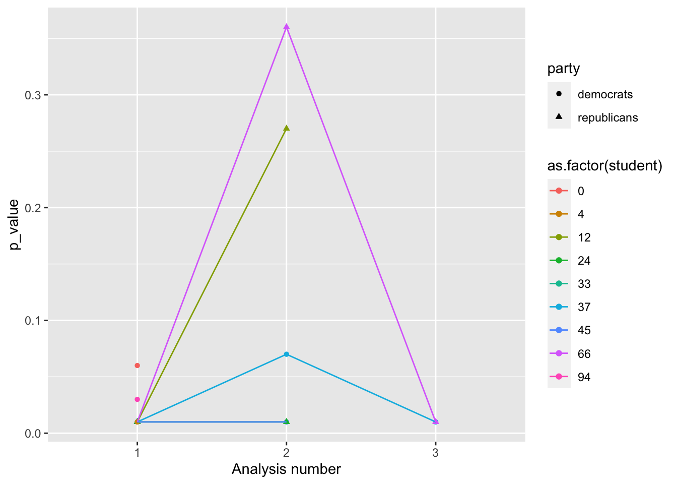
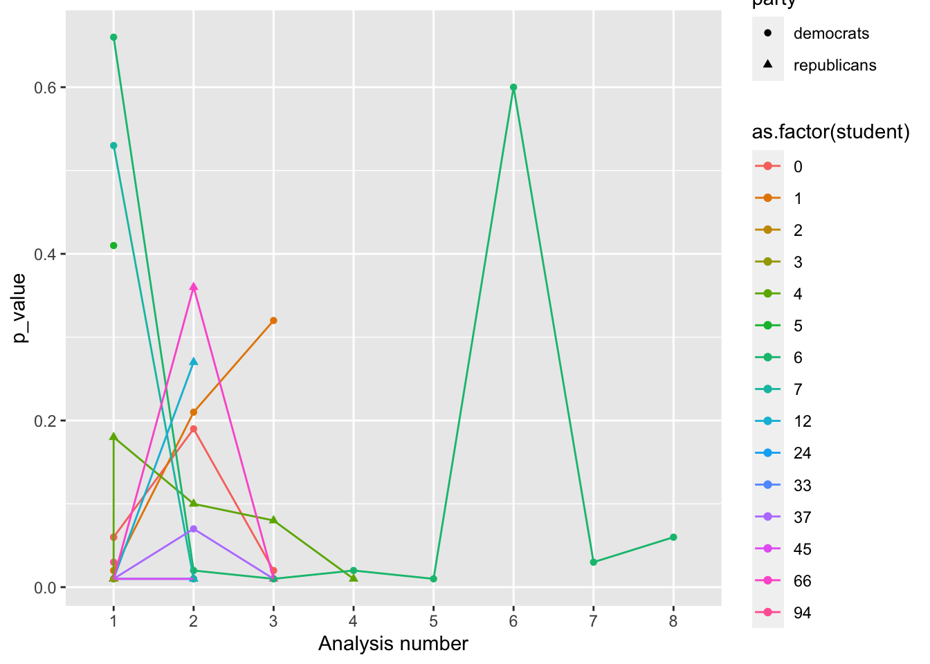
Figure 3: p-values by number of analyses: PSYCH 490 Fall 2023

How many different combinations of variables?

How many different combinations of variable choices are there?

There are \(n=4\) measures of political control; \(n=4\) measures of economic performance; \(n=2\) ‘other’ factors; \(n=2\) prediction choices; and \(n=2\) political parties to focus on.

We can use the combinat package to help us figure this out.

combinat::combn(c('pres', 'gov', 'senate', 'house'), 1)

     [,1]   [,2]  [,3]     [,4]   
[1,] "pres" "gov" "senate" "house"

This shows us the number of ways we can pick a single political measure from among the 4 choices. We see that there are 4 ways.

The next function shows us the number of ways to pick two measures.

combinat::combn(c('pres', 'gov', 'senate', 'house'), 2)

     [,1]   [,2]     [,3]    [,4]     [,5]    [,6]    
[1,] "pres" "pres"   "pres"  "gov"    "gov"   "senate"
[2,] "gov"  "senate" "house" "senate" "house" "house" 

There are 6 columns of two, so there must be 6 different ways to pick two measures.

combinat::combn(c('pres', 'gov', 'senate', 'house'), 3)

     [,1]     [,2]    [,3]     [,4]    
[1,] "pres"   "pres"  "pres"   "gov"   
[2,] "gov"    "gov"   "senate" "senate"
[3,] "senate" "house" "house"  "house" 

There are 4 different ways to pick 3 measures.

And there is only one way to pick 4 among 4. Make sense?

If we add these up ‘4 + 6 + 4 + 1’ = 15 we get the number of different choices we can make (15) about how many combinations of political power measures are possible.

Since there are also 4 different choices of economic performance measures, we know that there are 15 ways to pick these. Now we can calculate how many different possible combinations of variables there are.

n_combos <- 15*15*2*2*2

We multiply because each of the choices (political power, economic performance, party, better or worse is independent).

So, there are \(n=\) 1800 of variables we could have chosen. How does this impact the conclusions we can and should draw?

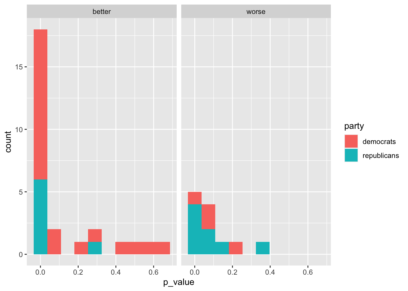
Combine with Spring 2023 data?

We did the same exercise in Spring 2023. Let’s combine our data with theirs.

googledrive::drive_download(file = "PSYCH 490.002 2023 P-hacking", path = "csv/p-hacking-sp23.csv", type = 'csv', overwrite = TRUE)

File downloaded:

• 'PSYCH 490.002 2023 P-hacking'
  <id: 1fnSwFrUcKvgqq_agDLe4t2DHXHtHoOlmLdtLVRSemrI>

Saved locally as:

• 'csv/p-hacking-sp23.csv'

p_hacking_sp23 <- read_csv(file = "csv/p-hacking-sp23.csv", show_col_types = FALSE)

p_hacking_sp23$semester = "sp23"
p_hacking_fa23$semester = "fa23"

p_hacking_23 <- rbind(p_hacking_fa23, p_hacking_sp23)

Combined data

p_hacking_23 |>
  ggplot() +
  aes(x = p_value, fill = party) +
  geom_histogram(bins = 10) +
  facet_grid(~ prediction)

p_hacking_23 |>
  ggplot() +
  aes(
    x = as.factor(analysis),
    y = p_value,
    color = as.factor(student),
    shape = party,
    group = as.factor(student)
  ) +
  geom_point() +
  geom_line() +
  xlab("Analysis number")

Choices for ‘political power’

power_df <- p_hacking_23 |>
  pivot_longer(cols = contains('power_'), 
                      names_to = "political_positions", 
                      values_to = "pol_pos_selected") |>
  distinct() |>
  mutate(political_positions = stringr::str_remove(string = political_positions,
                                                             pattern = "power_"))

power_df |> 
  dplyr::group_by(party, prediction, political_positions) |>
  dplyr::summarize(n_preds = sum(as.numeric(pol_pos_selected))) |>
  dplyr::arrange(desc(n_preds)) |>
  knitr::kable(format="html") |>
  kableExtra::kable_classic()

`summarise()` has grouped output by 'party', 'prediction'. You can override
using the `.groups` argument.

party	prediction	political_positions	n_preds
democrats	better	president	19
democrats	better	governors	12
democrats	better	reps	10
democrats	better	senators	10
republicans	better	reps	6
republicans	better	senators	6
republicans	better	president	5
republicans	worse	president	5
democrats	worse	reps	4
democrats	worse	senators	4
republicans	worse	reps	4
republicans	worse	senators	3
republicans	better	governors	2
republicans	worse	governors	2
democrats	worse	governors	0
democrats	worse	president	0

Figure 4: Respondents’ choices of political offices in their analyses

Choices for ‘economy’

econ_df <- p_hacking_23 |>
  pivot_longer(cols = contains('econ_'), 
                      names_to = "econ_measures", 
                      values_to = "econ_meas_selected") |>
  distinct() |>
  mutate(econ_measures = stringr::str_remove(string = econ_measures,
                                                             pattern = "econ_"))

econ_df |> 
  dplyr::group_by(party, prediction, econ_measures) |>
  dplyr::summarize(n_preds = sum(as.numeric(econ_meas_selected))) |>
  dplyr::arrange(desc(n_preds)) |>
  knitr::kable(format="html") |>
  kableExtra::kable_classic()

`summarise()` has grouped output by 'party', 'prediction'. You can override
using the `.groups` argument.

party	prediction	econ_measures	n_preds
democrats	better	employment	18
democrats	better	gdp	16
democrats	better	inflation	10
democrats	better	stocks	9
republicans	worse	employment	7
republicans	worse	gdp	6
republicans	worse	inflation	6
republicans	better	stocks	5
democrats	worse	employment	4
democrats	worse	stocks	4
republicans	better	employment	4
republicans	better	inflation	4
republicans	better	gdp	2
democrats	worse	gdp	0
democrats	worse	inflation	0
republicans	worse	stocks	0

Figure 5: Respondents’ choices of economic measures in their analyses

References

Wilkinson, M. D., Dumontier, M., Aalbersberg, I. J. J., Appleton, G., Axton, M., Baak, A., … Mons, B. (2016). The FAIR guiding principles for scientific data management and stewardship. Scientific Data, 3, 160018. https://doi.org/10.1038/sdata.2016.18